library(foreign); library(modelsummary)

gss <- droplevels(read.dta("https://tdmize.github.io/data/data/gss.dta"))

reg_op <- lm(occprest ~ age + income + woman + college + race, data = gss)

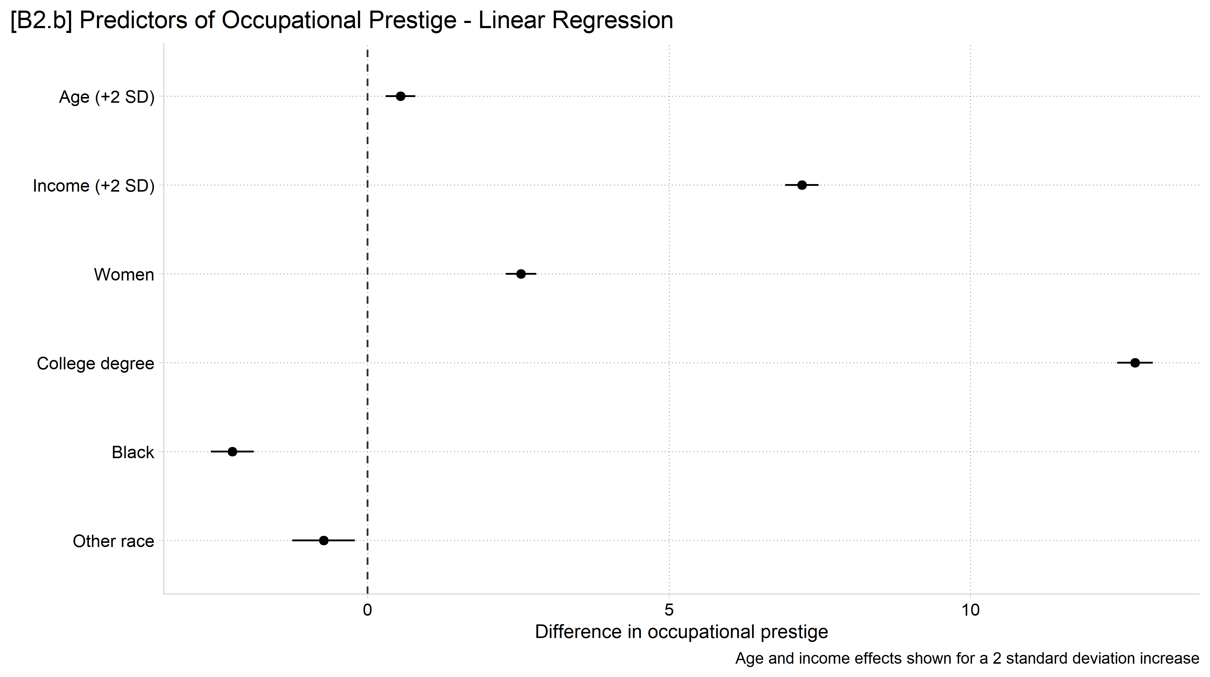
modelplot(reg_op)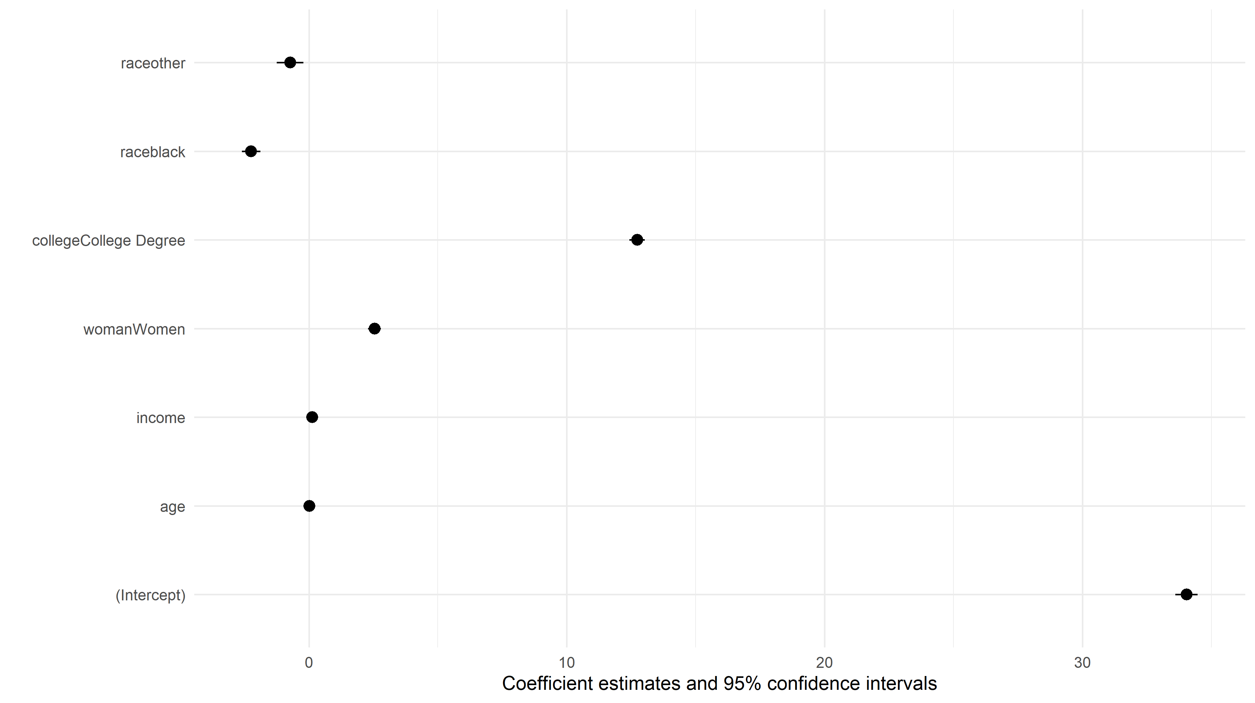
use "https://tdmize.github.io/data/data/gss.dta", clear(gss.dta | GSS 1972 - 2016 Data | DMV Workshop)regress occprest c.age c.income i.woman i.college i.race Source | SS df MS Number of obs = 36,381
-------------+---------------------------------- F(6, 36374) = 2648.96
Model | 2184216.72 6 364036.12 Prob > F = 0.0000
Residual | 4998736.44 36,374 137.426086 R-squared = 0.3041
-------------+---------------------------------- Adj R-squared = 0.3040
Total | 7182953.16 36,380 197.442363 Root MSE = 11.723
-------------------------------------------------------------------------------
occprest | Coefficient Std. err. t P>|t| [95% conf. interval]
--------------+----------------------------------------------------------------
age | 0.020 0.005 4.337 0.000 0.011 0.029
income | 0.129 0.003 51.304 0.000 0.124 0.134
|
woman |
Women | 2.544 0.129 19.721 0.000 2.291 2.797
|
college |
College De.. | 12.727 0.150 84.815 0.000 12.433 13.021
|
race |
black | -2.243 0.182 -12.317 0.000 -2.600 -1.886
other | -0.729 0.264 -2.757 0.006 -1.247 -0.211
|
_cons | 34.033 0.218 155.923 0.000 33.605 34.461
-------------------------------------------------------------------------------coefplot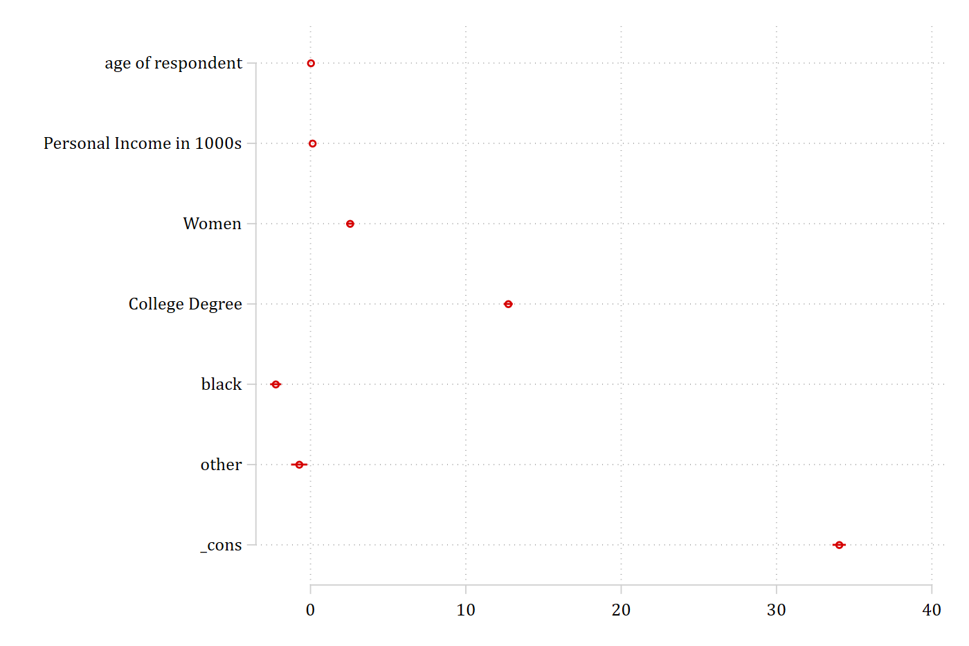
library(foreign); library(modelsummary)
gss <- droplevels(read.dta("https://tdmize.github.io/data/data/gss.dta"))
reg_op <- lm(occprest ~ age + income + woman + college + race, data = gss)
modelplot(reg_op)
Show effects of the continuous IVs for a 2 standard deviation increase
// B2.b - A publication-quality version
* Show effects of the continuous IVs for a 2 standard deviation increase
sum age if e(sample)
Variable | Obs Mean Std. dev. Min Max
-------------+---------------------------------------------------------
age | 36,381 40.82744 13.45085 18 89global age2sd = 2*r(sd)
sum income if e(sample) Variable | Obs Mean Std. dev. Min Max
-------------+---------------------------------------------------------
income | 36,381 31.36155 27.99743 .363 160global inc2sd = 2*r(sd)
coefplot, xline(0) baselevels ciop(col(*.6)) drop(_cons 0.woman) ///
rescale(age = $age2sd income = $inc2sd) ///
coeflabels(age = "Age (+2 SD)" income = "Income (+2 SD)") ///
xtitle("Difference in occupational prestige") ///
title("[B2.b] Predictors of Occupational Prestige - Linear Regression") //
/
note("Age and income effects shown for a 2 standard deviation increase")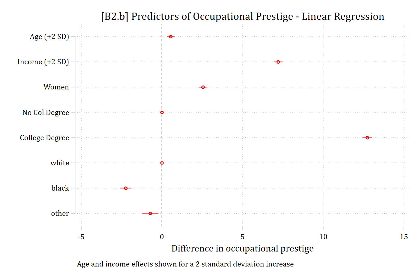
library(dplyr); library(ggplot2)
library(cleanplots)         # Mize's graphics scheme

## Use cleanplots colors, markers, lines, and theme for all graphs ##
cleanplots_defaults()
theme_update(plot.title.position = "plot")   # titles start at left edge of graph

# B2.b - A publication-quality version
# Show effects of the continuous IVs for a 2 standard deviation increase
gss_op <- filter(gss, !is.na(occprest), !is.na(age), !is.na(income), !is.na(woman),
                 !is.na(college), !is.na(race))
gss_op$age_2sd    <- gss_op$age / (2 * sd(gss_op$age))
gss_op$income_2sd <- gss_op$income / (2 * sd(gss_op$income))
reg_op2 <- lm(occprest ~ age_2sd + income_2sd + woman + college + race, data = gss_op)

modelplot(reg_op2, coef_omit = "Intercept",
          coef_rename = c("age_2sd" = "Age (+2 SD)", "income_2sd" = "Income (+2 SD)",
                          "womanWomen" = "Women",
                          "collegeCollege Degree" = "College degree",
                          "raceblack" = "Black", "raceother" = "Other race")) +
  geom_vline(xintercept = 0, linetype = "dashed", color = "gray20") +
  scale_y_discrete(limits = rev) +
  labs(x = "Difference in occupational prestige",
       title = "[B2.b] Predictors of Occupational Prestige - Linear Regression",
       caption = "Age and income effects shown for a 2 standard deviation increase")