3.6 Marginal Effects

Marginal effects defined: changes in probabilities

  • Note, in what follows η (“eta”) is denoting a prediction—almost always the predicted probability is of primary interest for binary logit/probit models
  • Compute probabilities at start and end values of xk

\[ME = \eta(x_{k} = end, \mathbf{x}_{-k} = \mathbf{x}^{*}) - \eta(x_{k} = start, \mathbf{x}_{-k} = \mathbf{x}^{*})\]

  • Starting and ending values of the focal IV \(x_{k}\) can be any values of substantive interest. For binary IVs, there are only two logical choices: 0 and 1

\[{ME}_{binary} = \eta(x_{k} = 1, \mathbf{x}_{-k} = \mathbf{x}^{*}) - \eta(x_{k} = 0, \mathbf{x}_{-k} = \mathbf{x}^{*})\]

  • For example, can compare a prediction for the non-religious (=0) to religious (=1)
  • For continuous IVs, many more choices for starting and ending values. Commonly:
    • start = mean of \(x_{k}\), or observed value
    • end = + 1 above start, + SD above start

Summarizing marginal effects

Review: Marginal effect at the mean (MEM)

  • The marginal effect at the mean (MEM) is the effect with all other variables in x-k (controls) at their means

\[MEM = \eta(x_{k} = end, \mathbf{x}_{-k} = \overline{\mathbf{x}}) - \eta(x_{k} = start, \mathbf{x}_{-k} = \overline{\mathbf{x}})\]

  • E.g., For a continuous variable (e.g. age) could compare predictions at the mean and at the mean + 1, with all controls (x-k) at means:

\[{MEM}_{continuous\ IV} = \eta(x_{k} = \overline{x}_{k} + 1, \mathbf{x}_{-k} = \overline{\mathbf{x}}) - \eta(x_{k} = \overline{x}_{k}, \mathbf{x}_{-k} = \overline{\mathbf{x}})\]

  • MEM interpretation is the effect on the probability for “the average person” or “someone who is average on all characteristics included in the model”

Review: Average marginal effect (AME)

  • We can compute a marginal effect for each observation in the data
    • Compute prediction at start (observed) and end (hypothetical change) values
    • The difference is the effect for that specific observation (MEi)*

\[{ME}_{i} = \eta(x_{k} = {end}_{i}, \mathbf{x}_{-k} = \mathbf{x}_{-k,i}) - \eta(x_{k} = {start}_{i}, \mathbf{x}_{-k} = \mathbf{x}_{-k,i})\]

  • Average marginal effect (AME) is the mean across all observations
    • Compute ME for each observation using observed values of x-k,i and average

\[AME = \frac{1}{N}\sum_{i = 1}^{N}\left\{\eta(x_{k} = {end}_{i}, \mathbf{x}_{-k} = \mathbf{x}_{-k,i}) - \eta(x_{k} = {start}_{i}, \mathbf{x}_{-k} = \mathbf{x}_{-k,i})\right\}\]

  • Interpretations of an AME is what the effect is “on average” in the sample
    • AMEs are my personal go-to default summary measure of an effect for categorical models
    • In my reading the AME is increasingly becoming the most popular method of interpretation across many fields

*See Appendix 3D for ways to examine the distribution of \({ME}_{i}\)s across a sample

Interpreting marginal effects for binary IVs

The examples use the GSS marijuana legalization model from 3.5:

use "https://tdmize.github.io/data/data/cda_gss22", clear
(GSS 1972-2022 CDA - Categorical Data Analysis | 2024-12-03)
drop if missing(grass, age, conserv, faminc, college, woman, race4)
(37,924 observations deleted)
recode grass 2 = 0
(0 changes made to grass)
lab def glab 0"not be legal" 1 "should be legal"
lab val grass glab
* Create year since 1975 variable
gen year1975 = year - 1975
lab var year1975 "years since 1975"
qui logit grass c.age c.year1975##c.year1975 i.conserv ///
    c.faminc i.degree i.woman i.race4, or
est store mjmod
* marginal effects for focal variables
mecompare conserv, models(mjmod)
Predicting: Pr(grass)
Marginal effects (N_mjmod=34466)

                                 |  ME #   Estimate         SE      P>|z|
---------------------------------+---------------------------------------
conserv                          |                                       
    Conservativ - Not Conser     |                                       
                           mjmod |     1     -0.153      0.005      0.000
library(haven)           # import Stata data and labels
library(dplyr)           # data manipulation
library(ggplot2)         # graphs
library(marginaleffects) # predictions and marginal effects
library(cleanplots)      # graph scheme
cleanplots_defaults()

source("https://raw.githubusercontent.com/tdmize/Rfunctions/main/ME_helper_functions.R")

# Center changes in continuous IVs on each observation's value
options(marginaleffects_contrast_direction = "center")

gss <- read_dta("https://tdmize.github.io/data/data/cda_gss22.dta")

# Drop any missing data on model vars
gss <- gss[complete.cases(gss[c("grass", "age", "conserv", "faminc", "college",
  "woman", "race4")]), ]

# Create year since 1975 variable; treat binary/nominal variables as factors
gss <- gss |>
  mutate(year1975 = as.numeric(year) - 1975,
    conserv = as_factor(conserv), degree = as_factor(degree),
    woman = as_factor(woman), race4 = as_factor(race4)) |>
  droplevels()

mjmod <- glm(grass ~ age + poly(year1975, 2, raw = TRUE) + conserv + faminc + degree +
  woman + race4, data = gss, family = binomial(link = "logit"))

# marginal effects for focal variables
avg_comparisons(mjmod, variables = "conserv")

 Estimate Std. Error     z Pr(>|z|)     S  2.5 % 97.5 %
   -0.153    0.00483 -31.7   <0.001 732.4 -0.163 -0.144

Term: conserv
Type: response
Comparison: Conservative - Not Conservative

On average, conservatives have a .15 lower probability of supporting marijuana legalization than do non-conservatives

Different wording:

Conservatives are about 15 percentage points less supportive of marijuana legalization, compared to non-conservatives

  • You may also want to report the actual conditional probabilities for each category of the binary IV, rather than just the difference out of context
    • Note you still want to refer to the significance test of the marginal effect. E.g.,
* show each predictions for each category of focal binary IV
est restore mjmod
(results mjmod are active now)
margins conserv
Predictive margins                                      Number of obs = 34,466
Model VCE: OIM

Expression: Pr(grass), predict()

-------------------------------------------------------------------------------
              |            Delta-method
              |     Margin   std. err.      z    P>|z|     [95% conf. interval]
--------------+----------------------------------------------------------------
      conserv |
Not Conser..  |      0.433      0.003  145.163   0.000        0.427       0.439
Conservative  |      0.279      0.004   74.284   0.000        0.272       0.287
-------------------------------------------------------------------------------
# show each predictions for each category of focal binary IV
avg_predictions(mjmod, variables = "conserv", by = "conserv")

          conserv Estimate Std. Error     z Pr(>|z|)   S 2.5 % 97.5 %
 Not Conservative    0.433    0.00298 145.2   <0.001 Inf 0.427  0.439
 Conservative        0.279    0.00376  74.3   <0.001 Inf 0.272  0.287

Type: response

The predicted probability of supporting marijuana legalization for non-conservatives is about 0.43 — compared to a significantly lower predicted probability of about 0.28 for conservatives (M.E. = -0.15 , p < 0.001)

Interpretation tip: To refer to a marginal effect, I often just use ME or M.E. in text. A capital ∆ (Delta) is another common notation.

Interpreting marginal effects for continuous IVs

  • For continuous IVs, can interpret a one-unit discrete change, a one standard deviation discrete change, or the instantaneous rate of change (slope)—or another custom \(\delta\) amount (e.g., +10 years of age)
    • I generally default to +SD absent a theoretically informed choice
sum age year1975
    Variable |        Obs        Mean    Std. dev.       Min        Max
-------------+---------------------------------------------------------
         age |     34,466    46.01648    17.19265         18         89
    year1975 |     34,466    23.55458    14.61027          0         47
mecompare age year1975, amount(sd) models(mjmod)
Predicting: Pr(grass)
Marginal effects (N_mjmod=34466)

                                 |  ME #   Estimate         SE      P>|z|
---------------------------------+---------------------------------------
age + SD (centered)              |                                       
                           mjmod |     1     -0.076      0.002      0.000
---------------------------------+---------------------------------------
year1975 + SD (centered)         |                                       
                           mjmod |     2      0.157      0.002      0.000
summary(gss[c("age", "year1975")])
      age           year1975    
 Min.   :18.00   Min.   : 0.00  
 1st Qu.:32.00   1st Qu.:12.00  
 Median :43.00   Median :23.00  
 Mean   :46.02   Mean   :23.55  
 3rd Qu.:59.00   3rd Qu.:37.00  
 Max.   :89.00   Max.   :47.00  
sd(gss$age)
[1] 17.19265
sd(gss$year1975)
[1] 14.61027
avg_comparisons(mjmod, variables = list(age = sd(gss$age), year1975 = sd(gss$year1975)))

     Term          Contrast Estimate Std. Error     z Pr(>|z|)     S   2.5 %  97.5 %
 age      +17.1926477284996  -0.0764    0.00246 -31.0   <0.001 698.2 -0.0812 -0.0716
 year1975 +14.6102673252095   0.1570    0.00237  66.3   <0.001   Inf  0.1524  0.1617

Type: response

On average, a standard deviation increase in age (about 17 years) is associated with being about 8 percentage points less supportive of marijuana legalization

Samples collected about 15 years later (\({ME}_{year + SD}\)), are about 16 percentage points more supportive of legalizing marijuana than earlier samples

Marginal effects at specific values of interest

  • Year is a variable with meaningful values
    • A SD increase is somewhat awkward for a year variable
    • Effects across the entire range or trimmed range (5th to 95th percentile) are informative here
mecompare year1975, amount(trimrange) models(mjmod)
Predicting: Pr(grass)
Marginal effects (N_mjmod=34466)

                                 |  ME #   Estimate         SE      P>|z|
---------------------------------+---------------------------------------
year1975(5-95%)                  |                                       
                           mjmod |     1      0.546      0.007      0.000
trimrange <- quantile(gss$year1975, c(.05, .95))
avg_comparisons(mjmod, variables = list(year1975 = trimrange))

 Estimate Std. Error    z Pr(>|z|)   S 2.5 % 97.5 %
    0.546    0.00708 77.2   <0.001 Inf 0.532   0.56

Term: year1975
Type: response
Comparison: 47 - 1

Support for marijuana legalization has changed dramatically over the years of the GSS. Since the question began being asked in 1975, to the latest survey in 2022, support for legalization has increased by almost 55 percentage points

AME vs MEM: Which should you use?

  • While MEMs and AMEs are usually quite similar in size, the MEM and AME are not identical for categorical DV models
* Compare AME vs MEM
mecompare age, amount(sd) models(mjmod) dec(5) atmeans // MEM
Predicting: Pr(grass)
Marginal effects (N_mjmod=34466)

                                 |  ME #   Estimate         SE      P>|z|
---------------------------------+---------------------------------------
age + SD (centered)              |                                       
                           mjmod |     1   -0.07862    0.00257    0.00000
mecompare age, amount(sd) models(mjmod) dec(5)         // AME
Predicting: Pr(grass)
Marginal effects (N_mjmod=34466)

                                 |  ME #   Estimate         SE      P>|z|
---------------------------------+---------------------------------------
age + SD (centered)              |                                       
                           mjmod |     1   -0.07640    0.00246    0.00000
# Compare AME vs MEM
comparisons(mjmod, variables = list(age = sd(gss$age)), newdata = "mean") # MEM

 Estimate Std. Error     z Pr(>|z|)     S  2.5 %  97.5 %
  -0.0863    0.00295 -29.3   <0.001 623.4 -0.092 -0.0805

Term: age
Type: response
Comparison: +17.1926477284996
avg_comparisons(mjmod, variables = list(age = sd(gss$age)))               # AME

 Estimate Std. Error   z Pr(>|z|)     S   2.5 %  97.5 %
  -0.0764    0.00246 -31   <0.001 698.2 -0.0812 -0.0716

Term: age
Type: response
Comparison: +17.1926477284996
  • Hanmer and Kalkan (2013 AJPS) show that there are situations where AME and MEM diverge and that the AME tends to perform better. However, in my experience they are almost identical and if you do find differences this is likely due to an idiosyncrasy in your data rather than a real substantive difference in the effect of your IV. Absent a meaningful difference between the two, I prefer the AME as the interpretation is more straightforward, less cumbersome, and more satisfying

Logit vs probit revisited: AMEs*

Correlation(logit, probit)
betas 0.9995
z-stat on beta 0.9980
AMEs 0.9997
z-stat on AMEs 0.9992
Ratio(logit / probit)
betas 1.7819
z-stat on beta 0.9816
AMEs 1.0269
z-stat on AMEs 1.0139
  • AMEs are all but identical across logit and probit
  • z statistics on AMEs are very similar across logit and probit
  • If predictions and/or marginal effects are of interest: the choice of whether to use logit or probit does not matter
    • The identifying assumption about the variance of the errors has almost no influence on predictions or marginal effects

*NOTE: The table above is based on the models predicting support for Trump shown earlier

Interpreting marginal effects for nominal IVs

* plot predictions for each category
est restore mjmod
(results mjmod are active now)
qui margins race4, post
coefplot, vertical ylab(.1(.1).5) ytitle("Pr(support legal marijuana)") ///
    title("[3.6.e] Probability of supporting marijuana legalization by race-et
hnicity (GSS)")

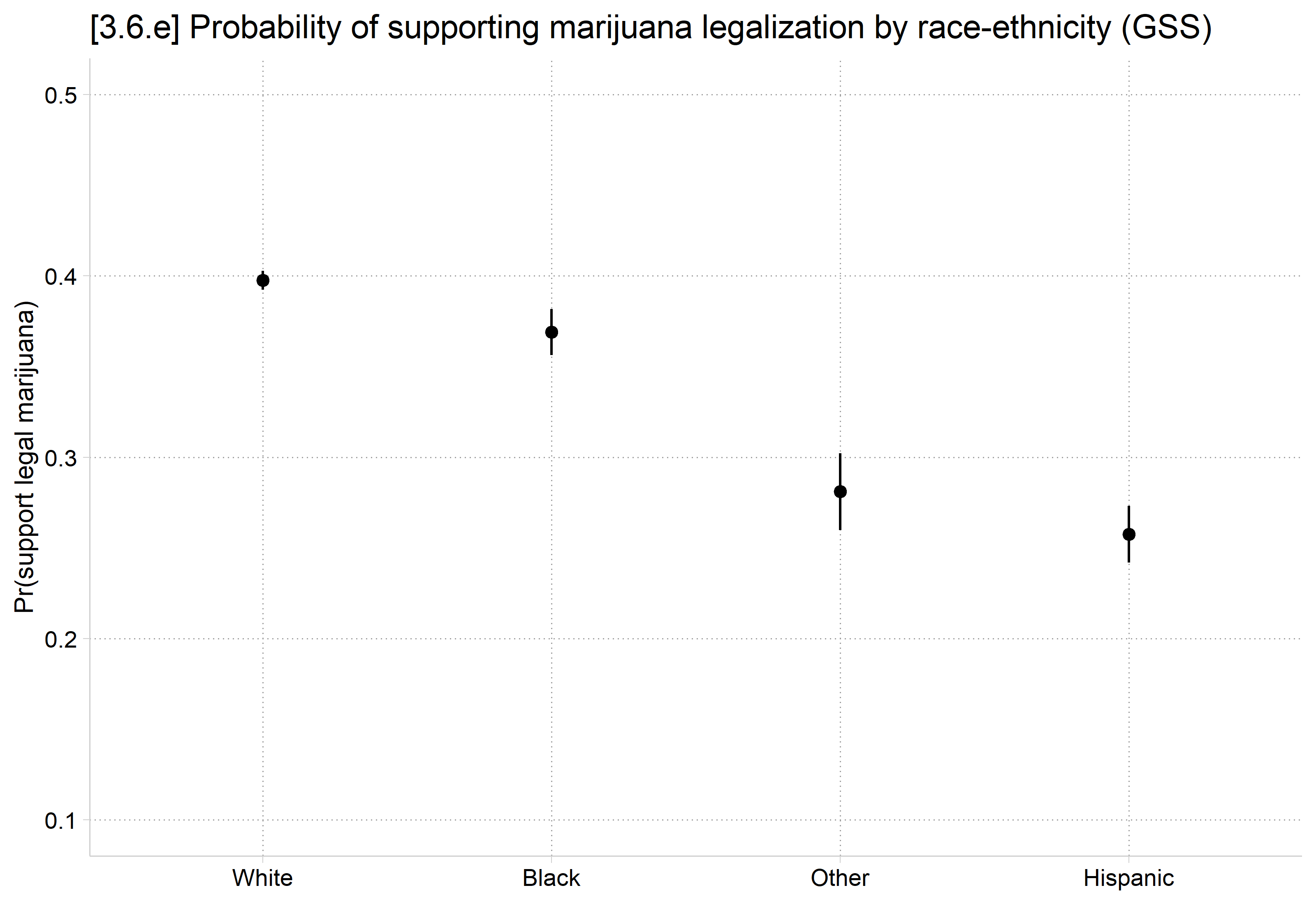
Predicted probability of supporting marijuana legalization by race-ethnicity with confidence intervals: about 0.40 for White, 0.37 for Black, 0.28 for Other, and 0.26 for Hispanic adults.

# plot predictions for each category
plot_predictions(mjmod, by = "race4",
  newdata = datagrid(race4 = unique, grid_type = "counterfactual")) +
  scale_y_continuous(breaks = seq(.1, .5, .1), limits = c(.1, .5)) +
  labs(title = "[3.6.e] Probability of supporting marijuana legalization by race-ethnicity (GSS)",
    x = NULL, y = "Pr(support legal marijuana)")

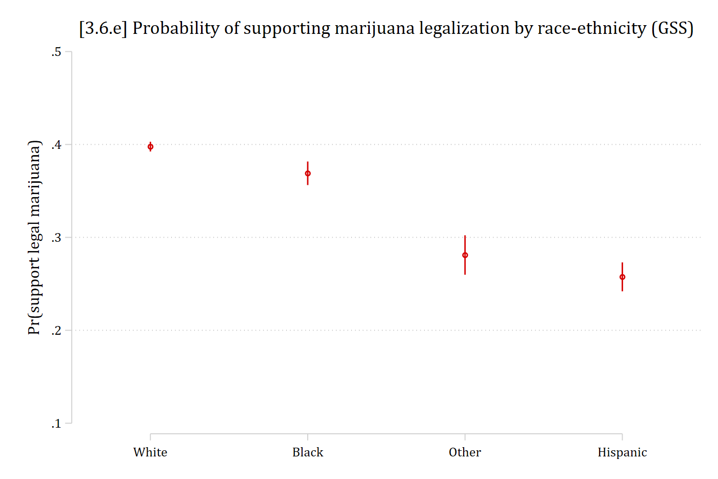
Predicted probability of supporting marijuana legalization by race-ethnicity with confidence intervals: about 0.40 for White, 0.37 for Black, 0.28 for Other, and 0.26 for Hispanic adults.

  • I always present the graph of predictions for a nominal IV, as it does not have a reference category / gives each group an equal amount of visual emphasis
  • The default interpretation for nominal IVs is generally to compare the prediction for each included category to an omitted reference category
    • But reference category is often arbitrary
    • And other contrasts are of interest
  • To avoid a reference category, compute all pairwise comparisons of predictions. Each pairwise comparison is a marginal effect

\[pairwise\ comparisons = ME = \eta(x_{k} = a, \mathbf{x}_{-k} = \mathbf{x}_{-k}^{*}) - \eta(x_{k} = b, \mathbf{x}_{-k} = \mathbf{x}_{-k}^{*});\ for\ all\ b > a\]

* ME pairwise comparisons
mecompare race4, models(mjmod) pwcompare
Predicting: Pr(grass)
Marginal effects (N_mjmod=34466)

                                 |  ME #   Estimate         SE      P>|z|
---------------------------------+---------------------------------------
race4                            |                                       
               Black - White     |                                       
                           mjmod |     1     -0.029      0.007      0.000
               Other - White     |                                       
                           mjmod |     2     -0.117      0.011      0.000
            Hispanic - White     |                                       
                           mjmod |     3     -0.140      0.008      0.000
               Other - Black     |                                       
                           mjmod |     4     -0.088      0.013      0.000
            Hispanic - Black     |                                       
                           mjmod |     5     -0.111      0.010      0.000
            Hispanic - Other     |                                       
                           mjmod |     6     -0.024      0.013      0.078
# ME pairwise comparisons
avg_comparisons(mjmod, variables = list(race4 = "pairwise"))

         Contrast Estimate Std. Error      z Pr(>|z|)     S   2.5 %   97.5 %
 Black - White     -0.0287    0.00704  -4.08   <0.001  14.4 -0.0425 -0.01490
 Hispanic - Black  -0.1115    0.01010 -11.04   <0.001  91.7 -0.1313 -0.09167
 Hispanic - Other  -0.0235    0.01333  -1.76   0.0778   3.7 -0.0496  0.00262
 Hispanic - White  -0.1402    0.00847 -16.55   <0.001 201.9 -0.1568 -0.12356
 Other - Black     -0.0879    0.01259  -6.98   <0.001  38.3 -0.1126 -0.06326
 Other - White     -0.1167    0.01117 -10.45   <0.001  82.5 -0.1385 -0.09477

Term: race4
Type: response

Black adults have slightly lower probabilities of supporting marijuana legalization than White adults, though the effect size is small (ME = -0.03)

Hispanic adults are about 14 percentage points less supportive of marijuana legalization than are White adults

Etc.

Marginal effects (ME) inequality

  • Issues with pairwise comparisons are many unhypothesized contrasts tested and no overarching answer about nominal IV’s effect size
  • The weighted ME inequality solves both issues (Mize and Han 2025)

\[ME\ inequality \equiv |weighted\ average\ ME\ inequality| = \sum_{a = 1}^{L}\sum_{b = 2;\ b > a}^{L}\frac{w_{a,b}}{L - 1} \left|\eta(x_{k} = a, \mathbf{x}_{-k} = \mathbf{x}_{-k}^{*}) - \eta(x_{k} = b, \mathbf{x}_{-k} = \mathbf{x}_{-k}^{*})\right|\]

  • Where \(w_{a,b}\) is a weight reflecting the sample sizes of each a and b category

In Stata, use the meinequality command or the meinequality option on mecompare

In R, use the meineq() function with avg_comparisons

* ME inequality
meinequality race4, models(mjmod)
ME Inequality Estimates (N = 34466)

                         |   Estimate   Std. err.           z       P>|z| 
-------------------------+-----------------------------------------------
ME Inequality            |                                               
                   race4 |      0.092       0.005      17.739       0.000 
# ME inequality
avg_comparisons(mjmod, variables = list(race4 = "pairwise"),
  hypothesis = meineq(mjmod))

 Estimate Std. Error    z Pr(>|z|)     S  2.5 % 97.5 %
   0.0919    0.00518 17.7   <0.001 231.5 0.0817  0.102

Term: race4
Type: response

Individuals from different racial-ethnic groups differ by about 9 percentage points, on average, in their support for legalizing marijuana (p < .001)

Summary of marginal effects

  • A summary measure of the “effect” of a variable is often useful
    • For linear additive effects in linear regression models the estimated coefficients are usually used (coefficient = ME; but only in this special case)
      • For nonlinear effects the regression coefficients do not directly indicate the magnitude of the effect in the natural metric of the DV
      • In the binary logit model odds ratios are often used, but are limited in their interpretability as discussed above
  • In most cases, measures of the change in the probability for a change in an IV (i.e., marginal effects) are the most helpful and intuitive way to summarize the effect
    • AME and MEM are generally almost identical; I prefer AME as a single measure in most cases due to its more elegant/satisfying interpretation
    • However, when there are meaningful or theoretically important values of your IVs to examine you should examine the effects at these values
      • Summary measures are only summaries and average over what may be important variation in the effect of interest
Back to top