Appendix A5: Stata Code and Tips

For all sets of lecture notes, there is an accompanying replication Stata do-file (available here or on Brightspace)
- This includes all of the Stata code necessary to recreate anything in the slides
In this Appendix, I include some comments, notes, and examples for things that are new or that might be hard to follow without more detail
For more streamlined, less complicated, and more notated do-files showing the basics of the types of analyses covered in this section, see the Assignment example code (also available on Brightspace)

A5.2 Marginal effects and plots of predictions

Predictions and plots of predictions for ordinal logit (ologit in Stata) use identical syntax as that for mlogit and are interpreted in the exact same way. E.g.

qui margins, at(year1972=(14(1)49))

marginsplot, noci … options … ///
    legend(order(1 "StrAgree" 2 "Agree" 3 "Disagree" 4 "StrDisag"))

Either margins or mchange can be used for calculating marginal effects. E.g.

mchange year1972, amount(sd)

Plotting predictions and marginal effects for nominal IVs

Plotting nominal IVs is exactly the same as in multinomial logit. There are two options:
- Plots of predictions for (1) each outcome category, and (2) each category of the nominal IV
- Plots of marginal effects

*Plots of predictions
est restore pillmod
margins, at(woman=0) post
est store Men
est restore pillmod
margins, at(woman=1) post
est store Women

coefplot (Men, color(eltblue)) (Women, color(red*1.2)), ///
    recast(bar) barw(0.2) vertical yline(0) ylab(0(.1).5) ///
    ciopts(recast(rcap) color(gs8)) citop scale(1.1)

*Plot of marginal effects
est restore pillmod
qui margins, dydx(woman)

marginsplot, recast(bar) ciopts(color(gs5)) ///
    xlab(0.5 " " 1 `" "Strongly" "Agree" "' 2 "Agree" ///
        3 "Disagree" 4 `" "Strongly" "Disagree" "' 4.5 " ") ///
    yline(0) plotopts(barw(0.6) color(ltblue))

A5.3 Plotting standardized coefficients

In Stata, you can use the coefplot command to plot coefficients from regression models
- I don’t recommend plotting odds ratios, especially not if you want to compare across models
  - +1 effect often not meaningful; effect size unclear; etc.
- But, plotting y* standardized coefficients can be useful
In Stata, there is no built-in way to plot standardized coefficients
- But, the transform( ) option allows you to standardize them manually
  - Specify * = @ / latentSD
  - Where the latentSD is that shown in listcoef, std (see 5.3)
- I always add an xline(0) with coefplots to easily see which effects are statistically significant
To fully (xy) standardize the continuous IVs, use the rescale option

use "https://tdmize.github.io/data/data/cda_gss", clear

(cda_gss.dta |  GSS 1972-2021 CDA - Categorical Data Analysis | date created 202
> 3)

*Reverse coded DV so interpretations are more natural
clonevar pillokR = pillok

(40,407 missing values generated)

lab def likrlab 1"StrDisag" 2"Disagree" 3"Agree" 4"StrAgree"
recode pillokR 1=4 2=3 3=2 4=1

(28,439 changes made to pillokR)

lab val pillokR likrlab
gen religous = attend

(665 missing values generated)

lab var religous "Religious Attendee"
recode religous 0/3 = 0 4/8 = 1

(55,475 changes made to religous)

lab def religlab 0"Not Religious" 1"Religious"
lab val religous religlab
drop if year < 1986

(18,586 observations deleted)

drop if missing(pillok, year1972, religous, college, age, woman, race3, faminc
)

(25,267 observations deleted)

qui ologit pillokR c.year1972 c.age i.woman i.religous ///
    i.college i.race3 c.faminc, or
est store pillmod
*Can use coefplot to plot estimates; need to specify transform option
*  and divide by Latent SD for y* standardized coefs
coefplot, transform(* = @/1.9105) xline(0) xlab(-.5(.1).5) ///
    title("[5.3.a] Support for birth control access for teenagers") ///
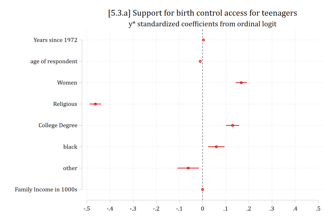
    subtitle("y* standardized coefficients from ordinal logit")
*To fully (xy) standardize continuous IVs, use the rescale option
coefplot, rescale(year1972 = 11.007 age = 17.164 faminc = 31.757) ///
    transform(* = @/1.9105) xline(0) xlab(-.5(.1).5) ///
    title("[5.3.b] Support for birth control access for teenagers") ///
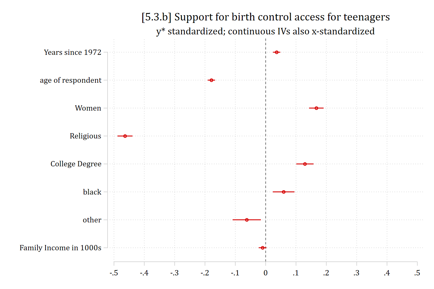
    subtitle("y* standardized; continuous IVs also x-standardized")

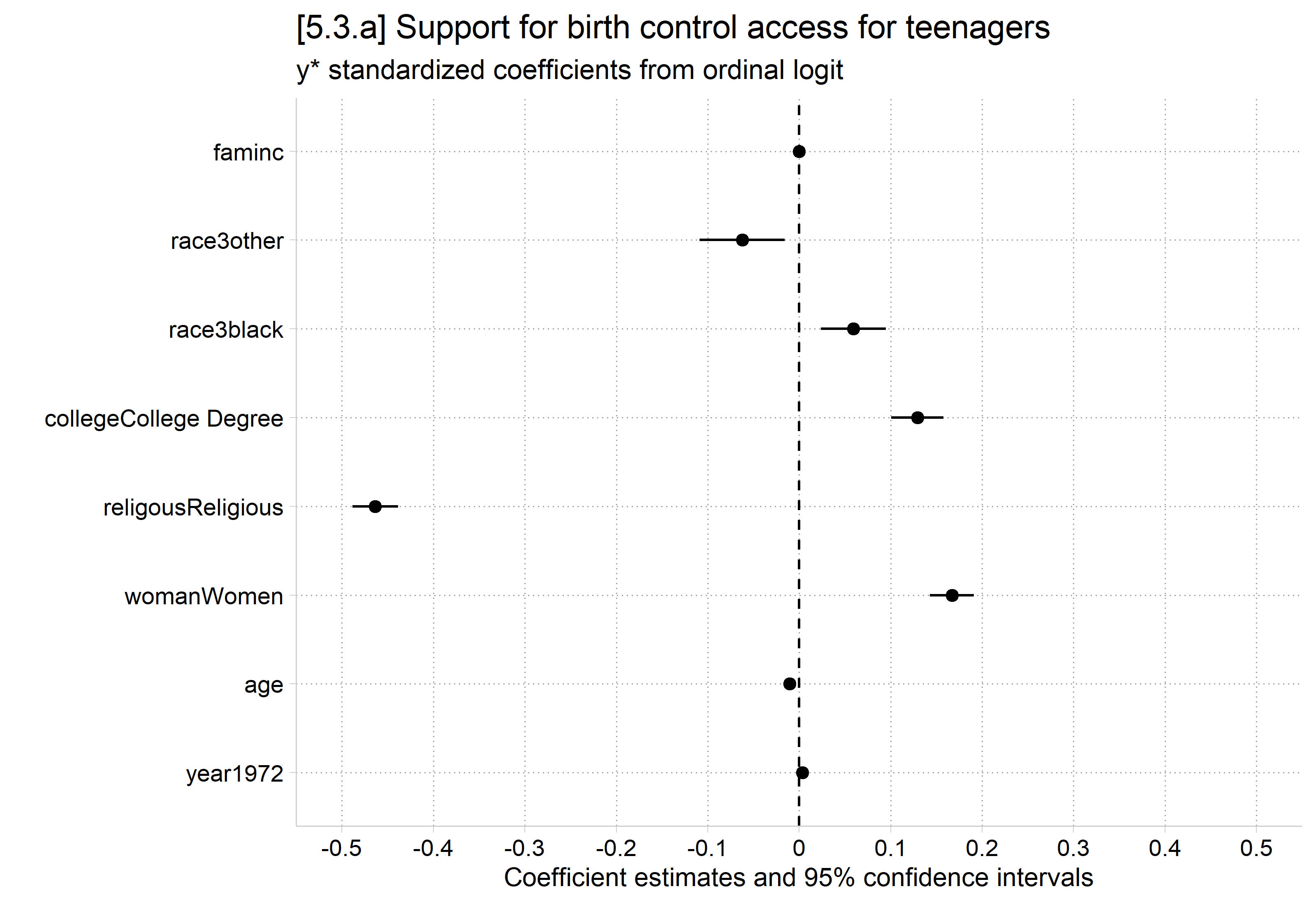
[5.3.a] Dot plot of y-star standardized coefficients from the ordinal logit with confidence intervals: religious about -0.46, other race about -0.06, women about 0.17, college degree about 0.13, Black about 0.06, and year, age, and family income near 0.

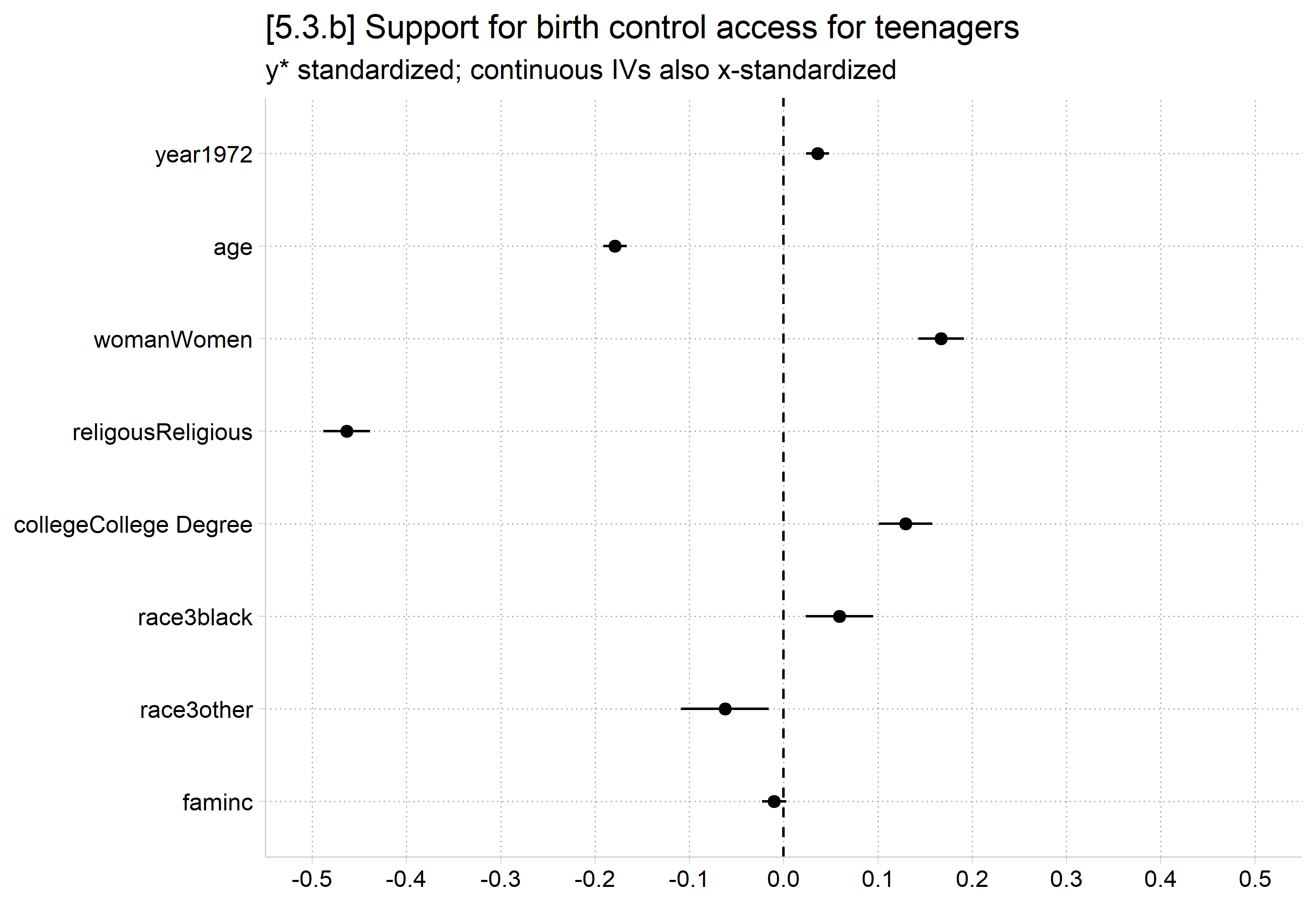
[5.3.b] Dot plot of the same coefficients with the continuous IVs also x-standardized: age is now about -0.18 and year about 0.04, with the other coefficients unchanged.

In R, use modelplot and specify a function() in scale_x_continuous that divides by the calculated SD of y*
- Add the zero null effect line as a geom_vline()

library(haven)           # import Stata data and labels
library(dplyr)           # data manipulation
library(ggplot2)         # graphs
library(MASS)            # ordinal logit: polr()
library(modelsummary)    # modelplot()
library(cleanplots)      # graph scheme
cleanplots_defaults()

gss <- read_dta("https://tdmize.github.io/data/data/cda_gss.dta")

# Religious attendee = attends about once a month or more
gss <- gss |>
  mutate(religous = case_when(attend <= 3 ~ 0, attend >= 4 ~ 1)) |>
  filter(year >= 1986)

# Keep model variables; drop any missing data
gss <- gss[c("pillok", "year1972", "religous", "college", "age", "woman", "race3", "faminc")]
gss <- gss[complete.cases(gss), ]

# Reverse coded DV so interpretations are more natural
gss <- gss |>
  mutate(pillokR = factor(5 - pillok, levels = 1:4,
      labels = c("StrDisag", "Disagree", "Agree", "StrAgree")),
    religous = factor(religous, labels = c("Not Religious", "Religious")),
    across(c(college, woman, race3), as_factor),
    year1972 = as.numeric(year1972)) |>
  droplevels()

pillmod <- polr(pillokR ~ year1972 + age + woman + religous + college + race3 + faminc,
  data = gss, Hess = TRUE)

# SD of y* (latent SD)
sdystar <- sqrt(var(pillmod$lp) + pi^2/3)

# 5.3.a: coefficients plotted on the axis of y* standardized coefficients
modelplot(pillmod, coef_omit = "\\|", ci_method = "wald") +
  scale_x_continuous(breaks = seq(-.5, .5, .1) * sdystar, limits = c(-.5, .5) * sdystar,
    labels = function(x) round(x / sdystar, 2)) +
  geom_vline(xintercept = 0, linetype = "dashed") +
  labs(title = "[5.3.a] Support for birth control access for teenagers",
    subtitle = "y* standardized coefficients from ordinal logit")

[5.3.a] Dot plot of y-star standardized coefficients from the ordinal logit with confidence intervals: religious about -0.46, other race about -0.06, women about 0.17, college degree about 0.13, Black about 0.06, and year, age, and family income near 0.

# 5.3.b: y* standardized; continuous IVs also x-standardized
std_coefs <- data.frame(term = names(coef(pillmod)), b = coef(pillmod),
  se = sqrt(diag(vcov(pillmod)))[names(coef(pillmod))]) |>
  mutate(sdx = case_when(term == "year1972" ~ sd(gss$year1972),
      term == "age" ~ sd(gss$age), term == "faminc" ~ sd(gss$faminc), TRUE ~ 1),
    estimate = b * sdx / sdystar,
    conf.low = (b - 1.96 * se) * sdx / sdystar,
    conf.high = (b + 1.96 * se) * sdx / sdystar,
    term = factor(term, levels = rev(term)))

ggplot(std_coefs, aes(x = estimate, y = term)) +
  geom_pointrange(aes(xmin = conf.low, xmax = conf.high)) +
  geom_vline(xintercept = 0, linetype = "dashed") +
  scale_x_continuous(breaks = seq(-.5, .5, .1), limits = c(-.5, .5)) +
  labs(title = "[5.3.b] Support for birth control access for teenagers",
    subtitle = "y* standardized; continuous IVs also x-standardized", x = NULL, y = NULL)

[5.3.b] Dot plot of the same coefficients with the continuous IVs also x-standardized: age is now about -0.18 and year about 0.04, with the other coefficients unchanged.