Appendix 4A: Combining Outcomes and Functional Forms

Testing that outcomes can be combined

  • Sometimes, you might want to combine outcome categories

    • E.g., You might think that the process you are studying is a binary outcome process even though it was measured as a nominal outcome
      • E.g., Although both “strongly agree” and “agree” were asked you think these could be combined
  • If the independent variables jointly have no effect on the odds of category 1 vs category 2, we say category 1 and category 2 are indistinguishable

  • The hypothesis that L and M are indistinguishable is

    \[H_{0}: \beta_{1,L|M} = \beta_{2,L|M} = \ldots = \beta_{k,L|M} = 0\]

    • I.e., That all of the IVs jointly considered have no significant predictive power as to whether an observation falls in category L or M

Wald tests for combining outcomes

  • Tests of indistinguishability can be computed for all pairs of outcomes
    • The SPost command mlogtest, combine will do this for you
use "https://tdmize.github.io/data/data/cda_gss", clear
(cda_gss.dta |  GSS 1972-2021 CDA - Categorical Data Analysis | date created 202
> 3)
keep if year >= 2016 & year <= 2021
(59,599 observations deleted)
drop if missing(conserv, age, woman, race3, college, married, parent, faminc)
(1,421 observations deleted)
*3 category political views var
qui mlogit polviews3 c.age i.woman i.race3 i.college ///
    i.married i.parent c.faminc i.employed
est store pol3mod
mlogtest, combine
Wald tests for combining alternatives (N=7823)

  Ho: All coefficients except intercepts associated with a given pair
      of alternatives are 0 (i.e., alternatives can be combined)

                 |      chi2    df   P>chi2
-----------------+-------------------------
Liberal & Mode~e |   379.293     9    0.000
Liberal & Cons~a |   455.146     9    0.000
Moderate & Con~a |   256.685     9    0.000
library(haven)           # import Stata data and labels
library(dplyr)           # data manipulation
library(sjmisc)          # frq() frequency tables
library(ggplot2)         # graphs
library(nnet)            # multinomial logit: multinom()
library(cleanplots)      # graph scheme
cleanplots_defaults()

gss <- read_dta("https://tdmize.github.io/data/data/cda_gss.dta")

gss <- gss |> filter(year >= 2016 & year <= 2021)

# Keep model variables; drop any missing data
gss <- gss[c("polviews3", "polviews", "age", "woman", "race3", "college", "married",
  "parent", "faminc", "income", "employed", "conserv", "year")]
gss <- gss[complete.cases(gss[c("conserv", "age", "woman", "race3", "college",
  "married", "parent", "faminc")]), ]

# Treat binary/nominal variables as factors
gss <- gss |>
  mutate(across(c(polviews3, woman, race3, college, married, parent, employed), as_factor)) |>
  droplevels()

# 3 category political views var
pol3mod <- multinom(polviews3 ~ age + woman + race3 + college + married + parent +
  faminc + employed, data = gss, trace = FALSE)

# Wald tests for combining each pair of outcomes (like mlogtest, combine):
# all coefficients except the intercepts are the same for the two outcomes
combine_tests <- function(model) {
  b <- coef(model)  # one row per outcome (other than the base outcome)
  V <- vcov(model)
  bvec <- setNames(as.vector(t(b)), colnames(V))
  outcomes <- model$lev
  terms <- colnames(b)[-1]
  pairs <- combn(outcomes, 2)
  out <- lapply(seq_len(ncol(pairs)), function(i) {
    o1 <- pairs[1, i]
    o2 <- pairs[2, i]
    # differences between the two outcomes' coefficients (base outcome = 0)
    L <- matrix(0, length(terms), length(bvec), dimnames = list(terms, names(bvec)))
    for (t in terms) {
      if (o1 != outcomes[1]) L[t, paste0(o1, ":", t)] <- 1
      if (o2 != outcomes[1]) L[t, paste0(o2, ":", t)] <- -1
    }
    d <- L %*% bvec
    chi2 <- as.numeric(t(d) %*% solve(L %*% V %*% t(L)) %*% d)
    data.frame(outcomes = paste(o1, "&", o2), chi2 = round(chi2, 3), df = length(terms),
      p = round(pchisq(chi2, length(terms), lower.tail = FALSE), 3))
  })
  do.call(rbind, out)
}

combine_tests(pol3mod)
                 outcomes    chi2 df p
1      Liberal & Moderate 379.293  9 0
2  Liberal & Conservative 455.142  9 0
3 Moderate & Conservative 256.682  9 0

We have evidence that we should not combine outcome categories; i.e., our model is able to distinguish between all three outcome categories.

Testing that outcomes can be combined: 7 categories

  • Consider a situation where we had more outcome categories. In fact, the GSS asks political views as a seven-category measure that I simplified into three for the examples above:
fre polviews
polviews -- think of self as liberal or conservative
-------------------------------------------------------------------------------
                                  |      Freq.    Percent      Valid       Cum.
----------------------------------+--------------------------------------------
Valid   1 extremely liberal       |        415       5.30       5.30       5.30
        2 liberal                 |       1123      14.35      14.35      19.65
        3 slightly liberal        |        954      12.19      12.19      31.84
        4 moderate, middle of the |       2791      35.66      35.66      67.51
          road                    |                                            
        5 slightly conservative   |       1019      13.02      13.02      80.53
        6 conservative            |       1189      15.19      15.19      95.72
        7 extremely conservative  |        335       4.28       4.28     100.00
        Total                     |       7826     100.00     100.00           
-------------------------------------------------------------------------------
frq(gss$polviews)
think of self as liberal or conservative (x) <numeric> 
# total N=7826 valid N=7826 mean=3.99 sd=1.52

Value |                        Label |    N | Raw % | Valid % | Cum. %
----------------------------------------------------------------------
    1 |            extremely liberal |  415 |  5.30 |    5.30 |   5.30
    2 |                      liberal | 1123 | 14.35 |   14.35 |  19.65
    3 |             slightly liberal |  954 | 12.19 |   12.19 |  31.84
    4 | moderate, middle of the road | 2791 | 35.66 |   35.66 |  67.51
    5 |        slightly conservative | 1019 | 13.02 |   13.02 |  80.53
    6 |                 conservative | 1189 | 15.19 |   15.19 |  95.72
    7 |       extremely conservative |  335 |  4.28 |    4.28 | 100.00
 <NA> |                         <NA> |    0 |  0.00 |    <NA> |   <NA>
  • Note I shortened the value labels below so they aren’t truncated to:

    1 = E_Lib, 2 = Lib, 3 = S_Lib, 4 = Mod, 5 = S_Cons, 6 = Cons, 7 = E_Cons

*Try 7 category political views var
clonevar polviews7 = polviews
lab def pol7lab 1"E_Lib" 2"Lib" 3"S_Lib" 4"Mod" ///
    5"S_Cons" 6"Cons" 7"E_Cons"
lab val polviews7 pol7lab
qui mlogit polviews7 c.age i.woman i.race3 i.college ///
    i.married i.parent c.income i.employed if year == 2016, rrr
mlogtest, combine
Wald tests for combining alternatives (N=1553)

  Ho: All coefficients except intercepts associated with a given pair
      of alternatives are 0 (i.e., alternatives can be combined)

                 |      chi2    df   P>chi2
-----------------+-------------------------
     E_Lib & Lib |     8.583     9    0.477
   E_Lib & S_Lib |    11.306     9    0.255
     E_Lib & Mod |    26.320     9    0.002
  E_Lib & S_Cons |    18.834     9    0.027
    E_Lib & Cons |    16.021     9    0.066
  E_Lib & E_Cons |    24.624     9    0.003
     Lib & S_Lib |    11.966     9    0.215
       Lib & Mod |    63.873     9    0.000
    Lib & S_Cons |    34.535     9    0.000
      Lib & Cons |    35.251     9    0.000
    Lib & E_Cons |    40.236     9    0.000
     S_Lib & Mod |    27.305     9    0.001
  S_Lib & S_Cons |    14.663     9    0.101
    S_Lib & Cons |    17.529     9    0.041
  S_Lib & E_Cons |    29.590     9    0.001
    Mod & S_Cons |    35.097     9    0.000
      Mod & Cons |    44.732     9    0.000
    Mod & E_Cons |    21.756     9    0.010
   S_Cons & Cons |    10.403     9    0.319
 S_Cons & E_Cons |    25.531     9    0.002
   Cons & E_Cons |    21.056     9    0.012
# Try 7 category political views var
gss <- gss |>
  mutate(polviews7 = factor(polviews, levels = 1:7,
    labels = c("E_Lib", "Lib", "S_Lib", "Mod", "S_Cons", "Cons", "E_Cons")))

# Income in $1,000s so R computes the standard errors accurately
# (the tests do not depend on the units of income)
pol7mod <- multinom(polviews7 ~ age + woman + race3 + college + married + parent +
  I(income / 1000) + employed, data = gss, subset = year == 2016,
  trace = FALSE, maxit = 500)

combine_tests(pol7mod)
          outcomes   chi2 df     p
1      E_Lib & Lib  8.582  9 0.477
2    E_Lib & S_Lib 11.302  9 0.256
3      E_Lib & Mod 26.316  9 0.002
4   E_Lib & S_Cons 18.835  9 0.027
5     E_Lib & Cons 16.025  9 0.066
6   E_Lib & E_Cons 24.633  9 0.003
7      Lib & S_Lib 11.964  9 0.215
8        Lib & Mod 63.873  9 0.000
9     Lib & S_Cons 34.534  9 0.000
10      Lib & Cons 35.253  9 0.000
11    Lib & E_Cons 40.238  9 0.000
12     S_Lib & Mod 27.303  9 0.001
13  S_Lib & S_Cons 14.661  9 0.101
14    S_Lib & Cons 17.527  9 0.041
15  S_Lib & E_Cons 29.589  9 0.001
16    Mod & S_Cons 35.098  9 0.000
17      Mod & Cons 44.734  9 0.000
18    Mod & E_Cons 21.760  9 0.010
19   S_Cons & Cons 10.402  9 0.319
20 S_Cons & E_Cons 25.536  9 0.002
21   Cons & E_Cons 21.059  9 0.012

A warning: Inconsistencies and over-fitting

  • The above tests suggest S_Cons = Cons
    • They also suggest S_Cons = S_Lib
      • Algebraically, this should mean Cons = S_Lib
      • However, this is not true (Cons = S_Lib rejected at p < 0.05)
  • Tests of hypotheses are not algebraic statements
    • Finding that one contrast suggests combining categories does not suggest that other contrasts will suggest the same
  • Tests for combining outcome categories can be useful to check whether a theoretically motivated reason for combining categories is also statistically justified
    • I recommend against blindly combining categories based on statistical criterion alone (would you combine slightly liberal and slightly conservative?)
    • Instead, these tests should generally be used as evidence for or against a theoretically reasonable combination of categories
  • Be careful not to over-fit your data
    • I.e., Even if you don’t find evidence that two categories can be distinguished in your specific model doesn’t mean those categories couldn’t be distinguished in other samples or in other model specifications

Nonlinear functional forms

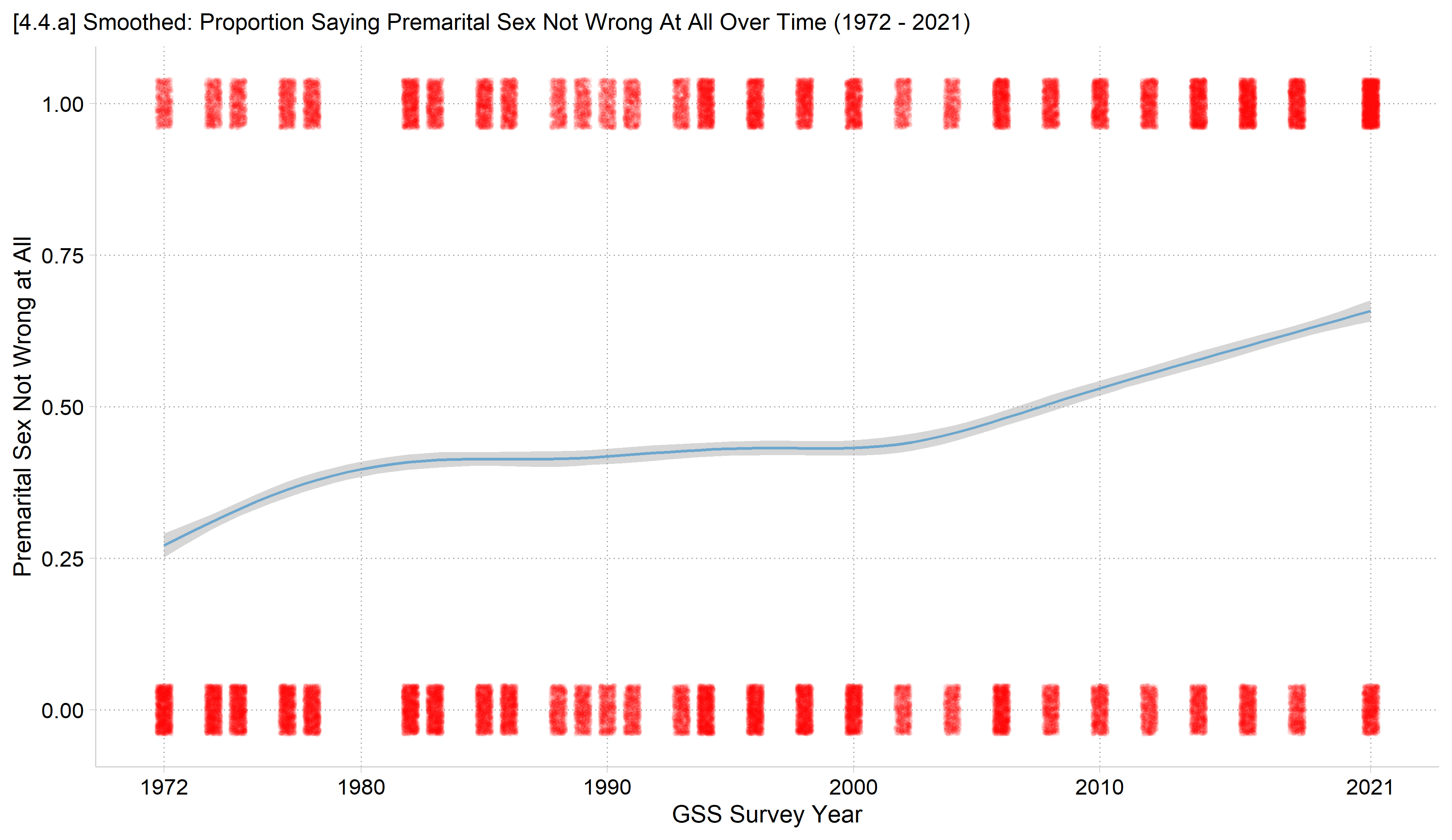
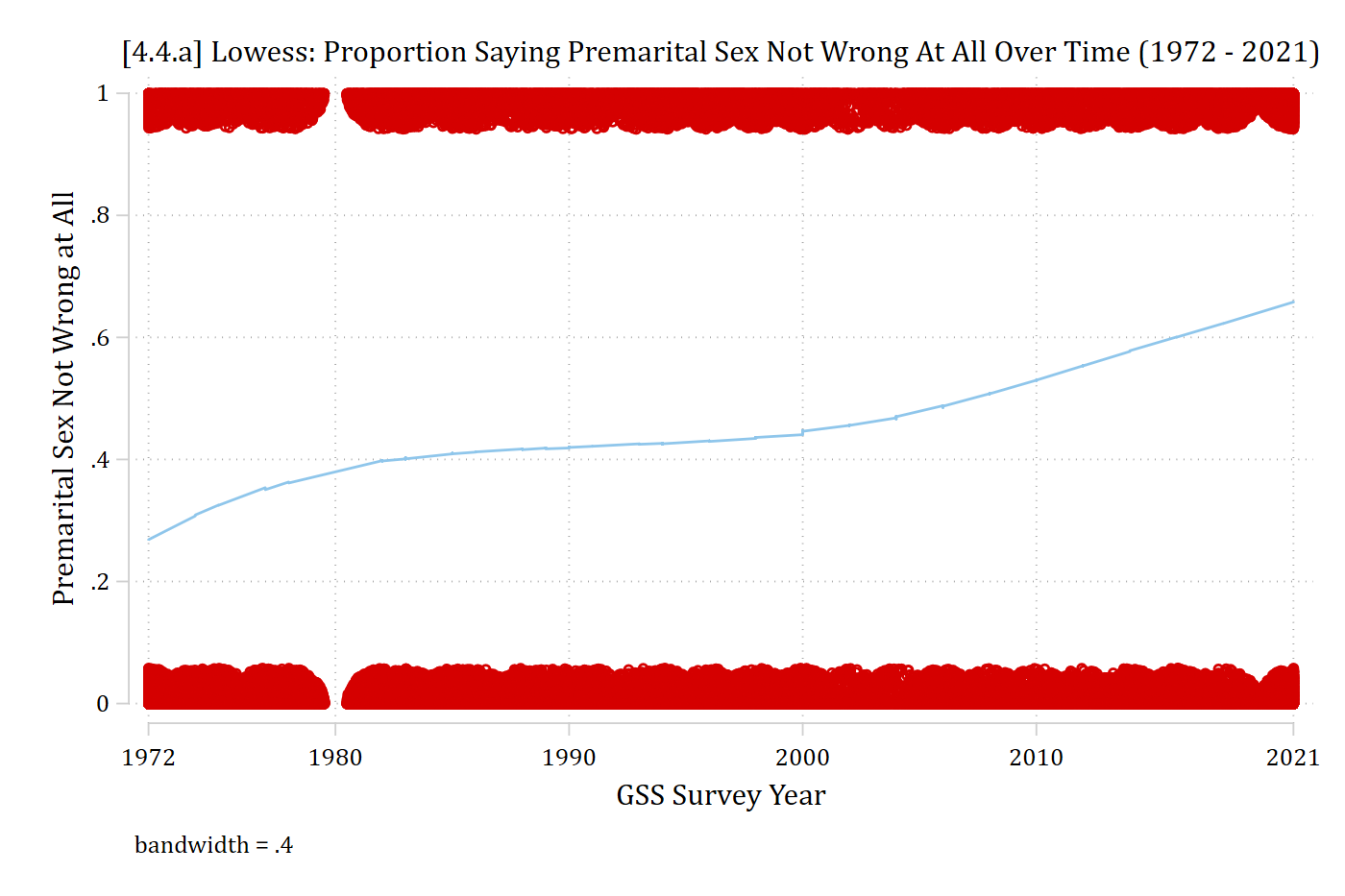
  • In exploratory analyses, I found time to have a functional form I did not expect the normal multinomial logit functional form to accommodate
  • The largest category “not wrong at all” appears to be the main culprit
  • Unfortunately, lowess doesn’t allow categorical DVs to assess functional form
  • An easy trick is to create a binary variable for the category you are examining with category of interest = 1; all others = 0
use "https://tdmize.github.io/data/data/cda_gss", clear
(cda_gss.dta |  GSS 1972-2021 CDA - Categorical Data Analysis | date created 202
> 3)
// Data cleaning //
gen religous = attend
(665 missing values generated)
lab var religous "Religious Attendee"
recode religous 0/3 = 0 4/8 = 1
(55,475 changes made to religous)
lab def religlab 0"Not Religious" 1"Religious"
lab val religous religlab
drop if missing(premarsx, college, age, woman, race3, year1972, religous)
(28,360 observations deleted)
*4.4.a - Lowess Plots to Assess Functional Form //
gen premarsxB = premarsx
lab var premarsxB "Premarital Sex Not Wrong at All"
recode premarsxB 1/3 = 0 4=1
(40,486 changes made to premarsxB)
lab def preblab 0"Wrong" 1"Not Wrong"
lab val premarsxB preblab
lowess premarsxB year1972, bwidth(0.4) jitter(8) ///
    xlab(0"1972" 8"1980" 18"1990" 28"2000" 38"2010" 49"2021") xtitle("GSS Surv
ey Year") ///
    title("[4.4.a] Lowess: Proportion Saying Premarital Sex Not Wrong At All O
ver Time (1972 - 2021)", size(medsmall))

[4.4.a] Lowess curve of the proportion saying premarital sex is not wrong at all, by GSS survey year, over jittered points at 0 and 1: it rises from about 0.27 in 1972 to about 0.40 by 1980, stays nearly flat around 0.40 to 0.45 until about 2000, then rises to about 0.66 in 2021.

gss <- read_dta("https://tdmize.github.io/data/data/cda_gss.dta")

# Data cleaning: religious attendee = attends about once a month or more
gss <- gss |>
  mutate(religous = case_when(attend <= 3 ~ 0, attend >= 4 ~ 1))

# Keep model variables; drop any missing data
gss <- gss[c("premarsx", "college", "age", "woman", "race3", "year1972", "religous")]
gss <- gss[complete.cases(gss), ]

# 4.4.a - Smoothed plot to assess functional form
gss <- gss |>
  mutate(premarsxB = ifelse(premarsx == 4, 1, 0),  # 1 = not wrong at all
    year1972 = as.numeric(year1972))

ggplot(gss, aes(x = year1972, y = premarsxB)) +
  geom_jitter(width = .3, height = .04, color = "red", alpha = .05, size = .5) +
  geom_smooth(color = "skyblue3") +
  scale_x_continuous(breaks = c(0, 8, 18, 28, 38, 49),
    labels = c("1972", "1980", "1990", "2000", "2010", "2021")) +
  labs(title = "[4.4.a] Smoothed: Proportion Saying Premarital Sex Not Wrong At All Over Time (1972 - 2021)",
    x = "GSS Survey Year", y = "Premarital Sex Not Wrong at All") +
  theme(plot.title.position = "plot", plot.title = element_text(size = rel(.9)))

[4.4.a] Smoothed curve of the proportion saying premarital sex is not wrong at all, by GSS survey year, over jittered points at 0 and 1: it rises from about 0.27 in 1972 to about 0.40 by 1980, stays nearly flat around 0.40 to 0.45 until about 2000, then rises to about 0.66 in 2021.

Difficult to guess specification needed in categorical models. Try year2 and also year3

BIC as a guide for specification of time*

*Examine BICs for different specifications of time
qui mlogit premarsx c.year1972 ///
    i.religous i.college c.age i.woman i.race3
est store year1
qui mlogit premarsx c.year1972##c.year1972 ///
    i.religous i.college c.age i.woman i.race3
est store year2
qui mlogit premarsx c.year1972##c.year1972##c.year1972 ///
    i.religous i.college c.age i.woman i.race3
est store year3
esttab year1 year2 year3, drop(*) bic ///
    title("Comparison of BICs for Various Specifications of Time") ///
    mtitles("Year^1" "Year^2" "Year^3")
Comparison of BICs for Various Specifications of Time
------------------------------------------------------------
                      (1)             (2)             (3)   
                   Year^1          Year^2          Year^3   
------------------------------------------------------------
------------------------------------------------------------
N                   40486           40486           40486   
BIC               90520.3         90517.6         90442.0   
------------------------------------------------------------
t statistics in parentheses
* p<0.05, ** p<0.01, *** p<0.001
# Treat binary/nominal variables as factors
gss <- gss |>
  mutate(across(c(premarsx, college, woman, race3), as_factor),
    religous = factor(religous, labels = c("Not Religious", "Religious"))) |>
  droplevels()

# Examine BICs for different specifications of time
# (year in decades inside the polynomials; the BICs are the same)
year1 <- multinom(premarsx ~ year1972 +
  religous + college + age + woman + race3, data = gss, trace = FALSE)
year2 <- multinom(premarsx ~ poly(I(year1972 / 10), 2, raw = TRUE) +
  religous + college + age + woman + race3, data = gss, trace = FALSE)
year3 <- multinom(premarsx ~ poly(I(year1972 / 10), 3, raw = TRUE) +
  religous + college + age + woman + race3, data = gss, trace = FALSE)

# Comparison of BICs for Various Specifications of Time
data.frame(model = c("Year^1", "Year^2", "Year^3"),
  N = nrow(gss), BIC = round(c(BIC(year1), BIC(year2), BIC(year3)), 1))
   model     N     BIC
1 Year^1 40486 90520.3
2 Year^2 40486 90517.6
3 Year^3 40486 90442.0

* From experience, I can say it is somewhat uncommon for the BIC to support such a complicated multinomial logit model because each additional polynomial adds J - 1 coefficients to the model; However the large sample size here (N > 40,000) likely affords us the statistical power for the more complicated model

Back to top