7.2 Testing for Interaction: Second Differences

Misinterpreting the interaction coefficient

  • Most people get this wrong and assume the coefficient on the interaction (product) terms tests the interaction in the predictions:
    • “A review of 13 economics journals listed on JSTOR found 72 articles published between 1980 and 1999 that used interaction terms in nonlinear models. None of the studies interpreted the coefficient on the interaction term correctly.” (Ai and Norton 2003 p.123)
    • “… I examined the 53 articles published in the American Sociological Review (ASR) between 2004 and 2016 examining nonlinear interaction effects. Fifty of the 53 referred only to the coefficient on the product term to determine the significance of the interaction effect—an improper test of interaction in terms of the predicted probabilities.” (Mize 2019 p.82)
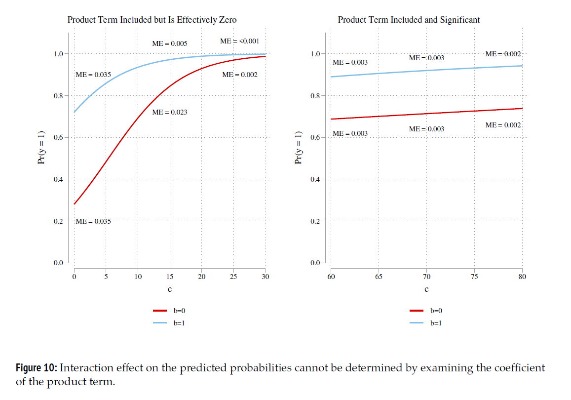
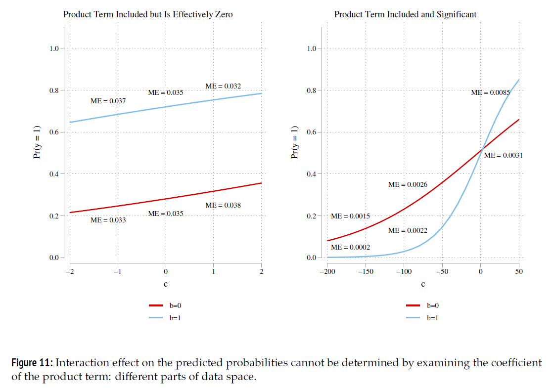
  • Plots below from Mize (2019) demonstrate how discrepant the effect on the predictions can be from the size and statistical significance of coefficient on the interaction (product) term

Figure 10 from Mize (2019): two panels of predicted probabilities for b = 0 and b = 1 across c. Left, the product term is included but is effectively zero, yet the marginal effects of c differ a lot between the groups (for example .035 versus .005). Right, the product term is included and significant, yet the marginal effects are nearly identical across the groups (.002 to .003). Caption: the interaction effect on the predicted probabilities cannot be determined by examining the coefficient of the product term.

Figure 11 from Mize (2019): the same two models plotted over different parts of the data space. Left, product term effectively zero: the lines for b = 0 and b = 1 are nearly parallel straight lines. Right, product term significant: the curves differ sharply and cross. Caption: the interaction effect on the predicted probabilities cannot be determined by examining the coefficient of the product term: different parts of data space.

Motivating example: Perceptions of love and support for formal rights and informal privileges for couples

Brian and Jennifer met three years ago and were immediately attracted to each other. After going on a few dates, Brian told Jennifer that he wanted to see her exclusively, to which Jennifer happily agreed; they’ve been together ever since. Although Brian and Jennifer have had serious arguments, they both report being happy when they are together. Brian and Jennifer feel complete trust in each other. In fact, they’ve lived together for the past two years.

Motivating example: couple type X love

  • Focal IV:
    • How in love do you think this couple is? (0 to 10 scale)
  • Moderating IV: Vignette random assigned couple type (sexuality) based on names:
    • Heterosexual couple; Lesbian couple; Gay couple
  • DVs:
    • Continuous scale: Are you supportive of informal privileges for this couple (e.g., talk about relationship with others; hold hands in public; kiss each other on cheek; etc.)?
    • Binary: Do you think they should be allowed to legally marry?
reg      informal i.cond##c.love10 … controls …

logit    marry i.cond##c.love10 … controls …
lm(informal ~ cond * love10 …)

glm(marry ~ cond * love10 … , family = binomial(link = "logit"))
use "https://tdmize.github.io/data/data/doan_love_SF", clear
(TESS03 - Analysis Dataset for TESS01 - Main Paper)
// Continuous DV: Informal Privileges //
qui reg informal i.cond##c.love10 rfem age rce_wht ed_coll ///
    ed_hs inc_50k married childyn children ideo evangel ///
    mainline blackprot catholic ofaithV2
est store inform
*7.2.a
qui margins, at(love10=(0(0.5)10) cond=(1 2 3))
marginsplot, recastci(rline) ciopt(lpat(dash) lcol(*.3)) xlab(0(2)10) ylab(0(2
)12) ///
    title("[7.2.a] Predicted Support of Informal Privileges by Perceptions of 
Love", size(medium)) ///
    subtitle("Effect of Sexual Orientation of Couple") ///
    ytitle("Predicted Approval") xtitle("Perceptions of Love") ///
    text(3 4 "Pr = 4.12" 9.5 4 "Pr = 8.06" 5.7 8 "Pr = 6.95" 11 8 "Pr = 9.81",
 size(small))
Variables that uniquely identify margins: love10 cond

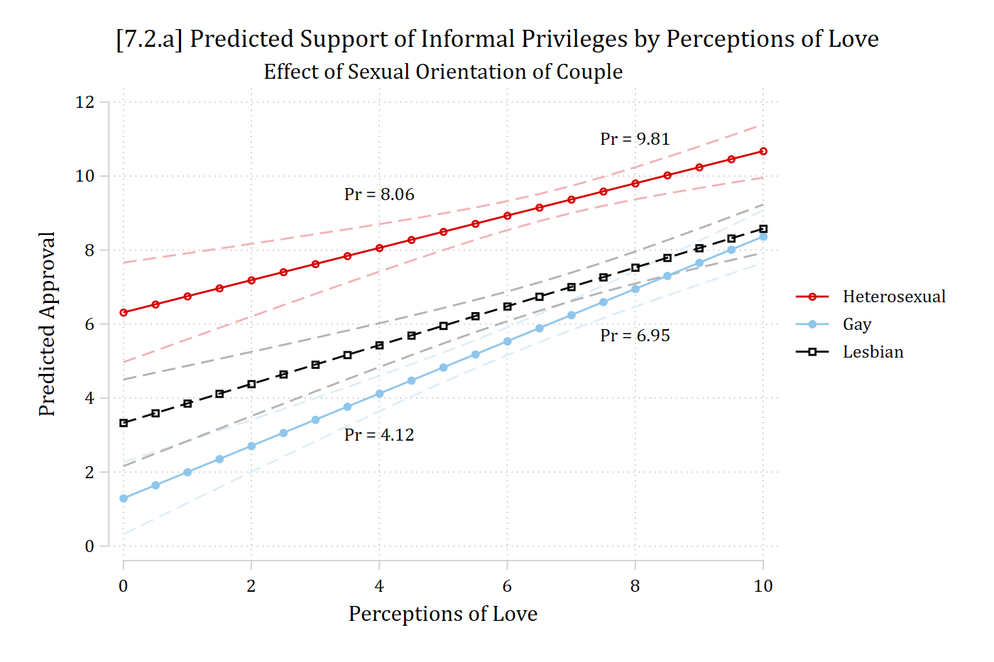
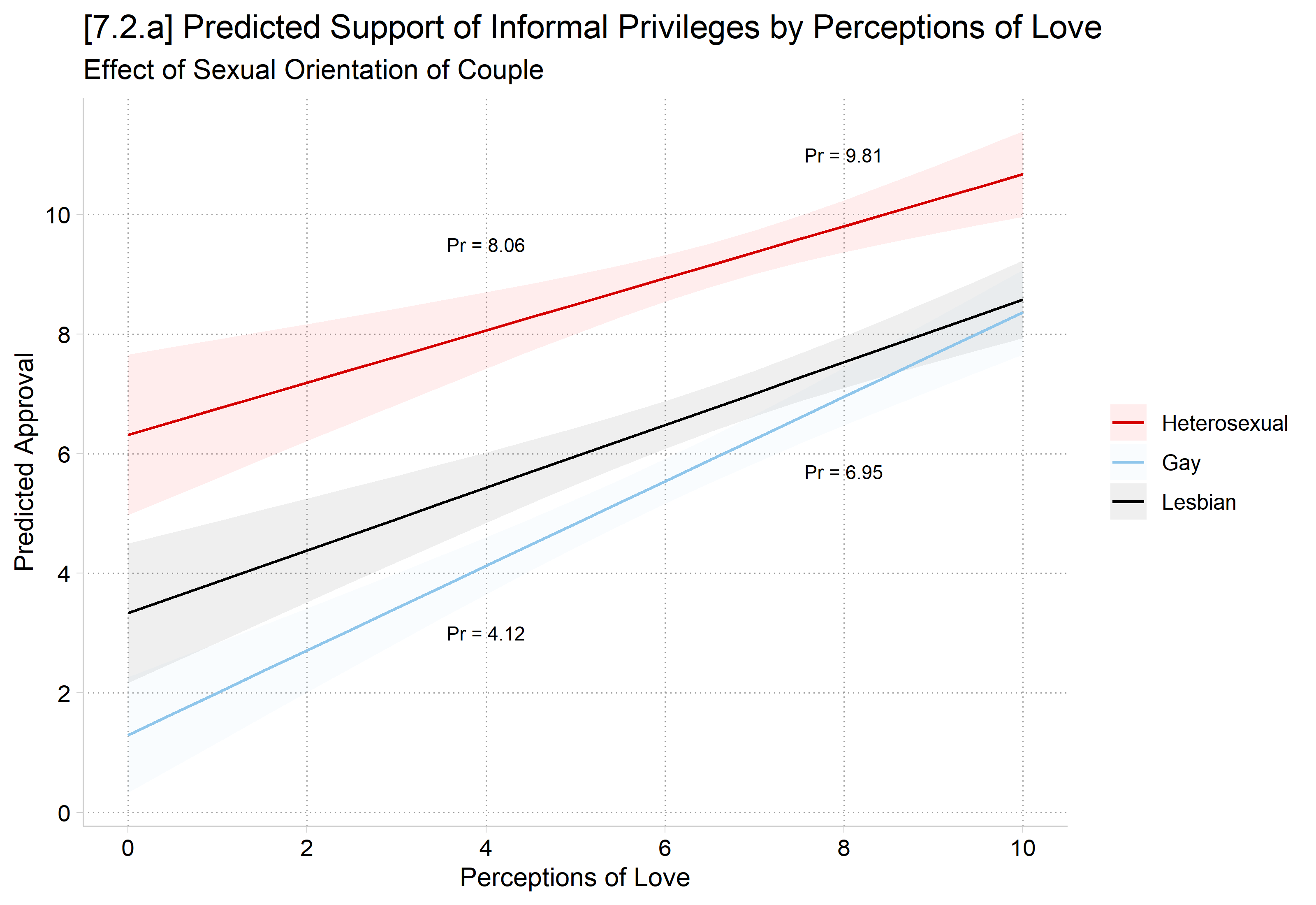
[7.2.a] Predicted support for informal privileges by perceptions of love (0 to 10) for heterosexual, gay, and lesbian couples, with confidence intervals. All three lines rise with love. The heterosexual line is highest, from about 6.3 to 10.7; the gay and lesbian lines start lower, near 1.3 and 3.3, and rise more steeply to about 8.4 and 8.6. Labels mark predictions of 8.06 and 9.81 for heterosexual couples and 4.12 and 6.95 for gay couples at love = 4 and 8.

library(haven)           # import Stata data and labels
library(dplyr)           # data manipulation
library(ggplot2)         # graphs
library(marginaleffects) # predictions and marginal effects
library(cleanplots)      # graph scheme
cleanplots_defaults()

love <- read_dta("https://tdmize.github.io/data/data/doan_love_SF.dta")

# Keep model variables; drop any missing data
love <- love[c("informal", "cond", "love10", "rfem", "age", "rce_wht", "ed_coll",
  "ed_hs", "inc_50k", "married", "childyn", "children", "ideo", "evangel",
  "mainline", "blackprot", "catholic", "ofaithV2")]
love <- love[complete.cases(love), ] |>
  mutate(cond = as_factor(cond))

# Continuous DV: Informal Privileges
inform <- lm(informal ~ cond * love10 + rfem + age + rce_wht + ed_coll + ed_hs +
  inc_50k + married + childyn + children + ideo + evangel + mainline + blackprot +
  catholic + ofaithV2, data = love)

# 7.2.a
plot_predictions(inform, by = c("love10", "cond"),
  newdata = datagrid(love10 = seq(0, 10, .5), cond = unique, grid_type = "counterfactual")) +
  annotate("text", x = c(4, 4, 8, 8), y = c(3, 9.5, 5.7, 11), size = 3,
    label = c("Pr = 4.12", "Pr = 8.06", "Pr = 6.95", "Pr = 9.81")) +
  scale_x_continuous(breaks = seq(0, 10, 2)) +
  scale_y_continuous(breaks = seq(0, 12, 2)) +
  labs(title = "[7.2.a] Predicted Support of Informal Privileges by Perceptions of Love",
    subtitle = "Effect of Sexual Orientation of Couple",
    x = "Perceptions of Love", y = "Predicted Approval", color = NULL, fill = NULL)
[7.2.a] Predicted support for informal privileges by perceptions of love (0 to 10) for heterosexual, gay, and lesbian couples, with confidence intervals. All three lines rise with love. The heterosexual line is highest, from about 6.3 to 10.7; the gay and lesbian lines start lower, near 1.3 and 3.3, and rise more steeply to about 8.4 and 8.6. Labels mark predictions of 8.06 and 9.81 for heterosexual couples and 4.12 and 6.95 for gay couples at love = 4 and 8.

1st Difference for Heterosexual Couple: 9.81 – 8.06 = 1.75

1st Difference for Gay Couple: 6.95 – 4.12 = 2.83

Testing 1st and 2nd differences with mtable and mlincom

*Predictions from 4 to 8
mtable, at(cond=(1 2) love10=(4 8)) post
Expression: Linear prediction, predict()

           |     cond    love10        xb
 ----------+-----------------------------
         1 |        1         4     8.061
         2 |        1         8     9.806
         3 |        2         4     4.124
         4 |        2         8     6.954

Specified values where .n indicates no values specified with at()

           |  No at()
 ----------+---------
   Current |       .n
*Effect of increase in love from 4 to 8 for Heterosexuals
mlincom 2 - 1, stat(est p)
             |   lincom    pvalue 
-------------+-------------------
           1 |    1.745     0.000 
*Effect of increase in love from 4 to 8 for Gay Men
mlincom 4 - 3, stat(est p)
             |   lincom    pvalue 
-------------+-------------------
           1 |    2.830     0.000 

In R, use avg_predictions and avg_comparisons

# Predictions from 4 to 8
avg_predictions(inform, by = c("cond", "love10"),
  newdata = datagrid(cond = c("Heterosexual", "Gay"), love10 = c(4, 8),
    grid_type = "counterfactual"))

         cond love10 Estimate Std. Error    z Pr(>|z|)     S 2.5 % 97.5 %
 Heterosexual      4     8.06      0.327 24.7   <0.001 444.6  7.42   8.70
 Heterosexual      8     9.81      0.221 44.4   <0.001   Inf  9.37  10.24
 Gay               4     4.12      0.243 16.9   <0.001 211.5  3.65   4.60
 Gay               8     6.95      0.246 28.3   <0.001 582.6  6.47   7.44

Type: response
# Effect of increase in love from 4 to 8 for Heterosexuals and Gay Men
fd <- avg_comparisons(inform, variables = list(love10 = c(4, 8)), by = "cond",
  newdata = datagrid(cond = c("Heterosexual", "Gay"), grid_type = "counterfactual"))
fd

         cond Estimate Std. Error    z Pr(>|z|)    S 2.5 % 97.5 %
 Heterosexual     1.74      0.390 4.47   <0.001 17.0 0.979   2.51
 Gay              2.83      0.305 9.27   <0.001 65.6 2.232   3.43

Term: love10
Type: response
Comparison: 8 - 4

This tells us that increases in perceptions of love from 4 to 8 have significant effects for both heterosexual and gay couples. But are these effects different?

  • A second difference is a test of whether two first differences are equal or not. Here, we have:
    • An effect (first difference) of love for heterosexual couples
    • An effect (first difference) of love for gay couples
      • Second difference = if effect is different for heterosexual and gay couples
  • From above, we know:
    • 1st difference for heterosexual couples = 1.745
    • 1st difference for gay couple = 2.830
      • 2nd difference = 2.830 – 1.745 = 1.085
*Does love have a stronger effect for gay men than heterosexuals?
mlincom (4 - 3) - (2 - 1), stat(est p)
             |   lincom    pvalue 
-------------+-------------------
           1 |    1.085     0.028 
# Does love have a stronger effect for gay men than heterosexuals?
hypotheses(fd, hypothesis = "b2 - b1 = 0")

 Hypothesis Estimate Std. Error    z Pr(>|z|)   S 2.5 % 97.5 %
    b2-b1=0     1.09      0.492 2.21   0.0273 5.2 0.122   2.05

Perceptions of love have a stronger effect on support for informal privileges for gay couples (∆gay = 2.830) than they do for heterosexual couples (∆heterosexual = 1.745; 2nd difference = 1.085; p < 0.05).

*And repeat for heterosexual vs lesbian, and gay vs lesbian

Back to top