5.3 Coefficients in the Ordinal Model

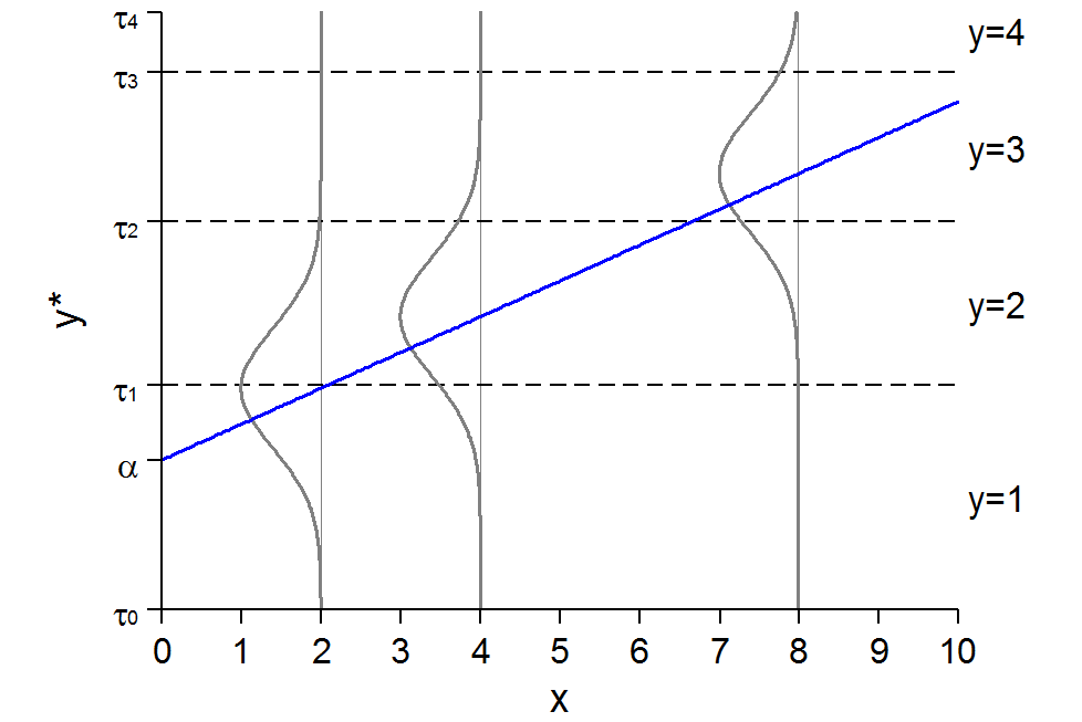
Latent y-star rising linearly with x, with normal error distributions drawn at x = 2, 4, and 8; dashed lines at the thresholds tau 1, tau 2, and tau 3 split each distribution into the probabilities of y = 1 to y = 4.

Cumulative probabilities in ordinal logit

  • The cumulative probability equals:

\[\Pr(y \leq j\,|\,\mathbf{x}) = \sum_{m = 1}^{j}\Pr(y = m\,|\,\mathbf{x})\]

For example

\[\begin{aligned} \Pr(SD\,|\,\mathbf{x}) &= \Pr(y = 1\,|\,\mathbf{x}) \\ \Pr(SD + D\,|\,\mathbf{x}) &= \Pr(y = 1\,|\,\mathbf{x}) + \Pr(y = 2\,|\,\mathbf{x}) \\ \Pr(SD + D + A\,|\,\mathbf{x}) &= \Pr(y = 1\,|\,\mathbf{x}) + \Pr(y = 2\,|\,\mathbf{x}) + \Pr(y = 3\,|\,\mathbf{x}) \end{aligned}\]

  • For SD + D + A

\[\begin{aligned} \Pr(SD + D + A\,|\,\mathbf{x}) &= \Pr(y \leq 3) \\ &= \Pr(y = 1\,|\,\mathbf{x}) + \Pr(y = 2\,|\,\mathbf{x}) + \Pr(y = 3\,|\,\mathbf{x}) \\ &= [\Lambda(\tau_{1} - \mathbf{x}_{i}\boldsymbol{\beta}) - \Lambda(\tau_{0} - \mathbf{x}_{i}\boldsymbol{\beta})] + [\Lambda(\tau_{2} - \mathbf{x}_{i}\boldsymbol{\beta}) - \Lambda(\tau_{1} - \mathbf{x}_{i}\boldsymbol{\beta})] \\ &\quad + [\Lambda(\tau_{3} - \mathbf{x}_{i}\boldsymbol{\beta}) - \Lambda(\tau_{2} - \mathbf{x}_{i}\boldsymbol{\beta})] \\ &= [\Lambda(\tau_{3} - \mathbf{x}_{i}\boldsymbol{\beta}) - \Lambda(\tau_{0} - \mathbf{x}_{i}\boldsymbol{\beta})] = \Lambda(\tau_{3} - \mathbf{x}_{i}\boldsymbol{\beta}) \end{aligned}\]

\[\Pr(y \leq j\,|\,\mathbf{x}) = \Lambda(\tau_{j} - \mathbf{x}\boldsymbol{\beta})\]

Cumulative probabilities in ordinal logit

  • This is a binary model with intercept \(\alpha_{j} = (\tau_{j} - \beta_{0})\) and slopes \(\boldsymbol{\beta}^{*} = -\boldsymbol{\beta}\)

\[\Pr(y \leq j\,|\,\mathbf{x}) = \Lambda(\tau_{j} - \mathbf{x}\boldsymbol{\beta}) = \Lambda(\alpha_{j} - \mathbf{x}\boldsymbol{\beta}^{*})\]

  • The odds of y ≤ j versus y > j given x are

\[\Omega_{j}(\mathbf{x}) = \frac{\Pr(y \leq j\,|\,\mathbf{x})}{\Pr(y > j\,|\,\mathbf{x})} = \exp(\tau_{j} - \mathbf{x}\boldsymbol{\beta}) = \exp(\alpha_{j} - \mathbf{x}\boldsymbol{\beta})\]

  • The odds ratio for a change in xk

\[\frac{\Omega_{j}(\mathbf{x}, x_{k} + 1)}{\Omega_{j}(\mathbf{x}, x_{k})} = \exp(\beta_{k}^{*})\]

Interpretation:

For a unit increase in xk the odds of higher outcomes compared to lower outcomes change by a factor of \(\exp(\beta_{k}^{*})\), holding other variables constant

Odds ratios interpretations in ordinal models

  • The odds are identical regardless where you binarize the comparison:

\[\Omega\left(\frac{P(SD)}{P(D, A, SA)}\right) = \Omega\left(\frac{P(SD, D)}{P(A, SA)}\right) = \Omega\left(\frac{P(SD, D, A)}{P(SA)}\right)\]

  • The odds ratio is interpreted in terms of the underlying latent variable (y*)
  • Effective interpretations are contingent on being able to properly and clearly name and talk about this underlying latent variable
    • Remember this must be a single unidirectional latent concept to satisfy the assumptions of the model
  • If you cannot easily or effectively decide what the latent variable is this is a pretty good indicator an ordinal model might not be appropriate

Naming the latent variable y*

  • How would you name and talk about the latent variable y* if you used one of the following ordinal variables as a DV?
    • All examples from the General Social Survey (GSS) which mostly consists of questions asked as ordinal variables

Would you say your own health, in general, is excellent, good, fair, or poor?

How often do you read the newspaper — every day, a few times a week, once a week, less than once a week, or never?

Because of past discrimination, employers should make special efforts to hire and promote qualified women…please tell me whether you strongly agree, agree, neither agree nor disagree, disagree, or strongly disagree.

Methods of birth control should be available to teenagers between the ages of 14 and 16 even if their parents do not approve… strongly agree, agree, disagree, or strongly disagree.

  • Good practice is to code your dependent variable in a way that will aid interpretation: higher numbers should = more of the latent construct

Odds ratios interpretations in ordinal models

I reverse coded the DV so that higher #s indicate more agreement for more natural interpretations

use "https://tdmize.github.io/data/data/cda_gss", clear
(cda_gss.dta |  GSS 1972-2021 CDA - Categorical Data Analysis | date created 202
> 3)
*Reverse coded DV so interpretations are more natural
clonevar pillokR = pillok
(40,407 missing values generated)
lab def likrlab 1"StrDisag" 2"Disagree" 3"Agree" 4"StrAgree"
recode pillokR 1=4 2=3 3=2 4=1
(28,439 changes made to pillokR)
lab val pillokR likrlab
gen religous = attend
(665 missing values generated)
lab var religous "Religious Attendee"
recode religous 0/3 = 0 4/8 = 1
(55,475 changes made to religous)
lab def religlab 0"Not Religious" 1"Religious"
lab val religous religlab
drop if year < 1986
(18,586 observations deleted)
drop if missing(pillok, year1972, religous, college, age, woman, race3, faminc
)
(25,267 observations deleted)
fre pillokR
pillokR -- birth control to teenagers 14-16
----------------------------------------------------------------
                   |      Freq.    Percent      Valid       Cum.
-------------------+--------------------------------------------
Valid   1 StrDisag |       4404      17.62      17.62      17.62
        2 Disagree |       5588      22.36      22.36      39.98
        3 Agree    |       7968      31.88      31.88      71.86
        4 StrAgree |       7033      28.14      28.14     100.00
        Total      |      24993     100.00     100.00           
----------------------------------------------------------------
ologit pillokR c.year1972 c.age i.woman i.religous ///
    i.college i.race3 c.faminc, or
Iteration 0:  Log likelihood = -34042.826  
Iteration 1:  Log likelihood = -32738.626  
Iteration 2:  Log likelihood = -32731.234  
Iteration 3:  Log likelihood =  -32731.23  
Iteration 4:  Log likelihood =  -32731.23  

Ordered logistic regression                            Number of obs =  24,993
                                                       LR chi2(8)    = 2623.19
                                                       Prob > chi2   =  0.0000
Log likelihood = -32731.23                             Pseudo R2     =  0.0385

-------------------------------------------------------------------------------
      pillokR | Odds ratio   Std. err.      z    P>|z|     [95% conf. interval]
--------------+----------------------------------------------------------------
     year1972 |      1.006      0.001    5.827   0.000        1.004       1.008
          age |      0.980      0.001  -28.640   0.000        0.979       0.982
              |
        woman |
       Women  |      1.376      0.032   13.628   0.000        1.314       1.441
              |
     religous |
   Religious  |      0.412      0.010  -36.615   0.000        0.393       0.432
              |
      college |
College De..  |      1.280      0.036    8.892   0.000        1.212       1.352
              |
        race3 |
       black  |      1.120      0.039    3.250   0.001        1.046       1.199
       other  |      0.888      0.040   -2.623   0.009        0.812       0.970
              |
       faminc |      0.999      0.000   -1.545   0.122        0.999       1.000
--------------+----------------------------------------------------------------
        /cut1 |     -2.556      0.051                        -2.657      -2.456
        /cut2 |     -1.334      0.049                        -1.431      -1.238
        /cut3 |      0.120      0.048                         0.025       0.215
-------------------------------------------------------------------------------
Note: Estimates are transformed only in the first equation to odds ratios.
est store pillmod
library(haven)           # import Stata data and labels
library(dplyr)           # data manipulation
library(sjmisc)          # frq() frequency tables
library(ggplot2)         # graphs
library(MASS)            # ordinal logit: polr()
library(marginaleffects) # predictions
library(cleanplots)      # graph scheme
cleanplots_defaults()

gss <- read_dta("https://tdmize.github.io/data/data/cda_gss.dta")

# Religious attendee = attends about once a month or more
gss <- gss |>
  mutate(religous = case_when(attend <= 3 ~ 0, attend >= 4 ~ 1)) |>
  filter(year >= 1986)

# Keep model variables; drop any missing data
gss <- gss[c("pillok", "year1972", "religous", "college", "age", "woman", "race3", "faminc")]
gss <- gss[complete.cases(gss), ]

# Reverse coded DV so interpretations are more natural
gss <- gss |>
  mutate(pillokR = factor(5 - pillok, levels = 1:4,
      labels = c("StrDisag", "Disagree", "Agree", "StrAgree")),
    religous = factor(religous, labels = c("Not Religious", "Religious")),
    across(c(college, woman, race3), as_factor),
    year1972 = as.numeric(year1972)) |>
  droplevels()

frq(gss$pillokR)
x <categorical> 
# total N=24993 valid N=24993 mean=2.71 sd=1.06

Value    |    N | Raw % | Valid % | Cum. %
------------------------------------------
StrDisag | 4404 | 17.62 |   17.62 |  17.62
Disagree | 5588 | 22.36 |   22.36 |  39.98
Agree    | 7968 | 31.88 |   31.88 |  71.86
StrAgree | 7033 | 28.14 |   28.14 | 100.00
<NA>     |    0 |  0.00 |    <NA> |   <NA>
pillmod <- polr(pillokR ~ year1972 + age + woman + religous + college + race3 + faminc,
  data = gss, Hess = TRUE)

# Odds ratios
exp(coef(pillmod))
             year1972                   age            womanWomen     religousReligious 
            1.0062935             0.9802916             1.3759937             0.4124401 
collegeCollege Degree            race3black            race3other                faminc 
            1.2803527             1.1198762             0.8878170             0.9993950 
# Thresholds (cuts)
pillmod$zeta
StrDisag|Disagree    Disagree|Agree    Agree|StrAgree 
       -2.5562557        -1.3340805         0.1201841 
  • For these interpretations I am using terminology for the latent variable y* for the DV “less to more supportive of access to birth control:”

Each year since this question was first asked, the odds of being more supportive has increased by a factor of 1.006

A year increase in age decreases the odds of supporting birth control for teenagers by a factor of about 0.98

Women’s odds of having supportive attitudes for teenage birth control access are higher than men’s by a factor of about 1.38

Religious individuals’ odds of supporting teenage birth control access is 0.41 times lower than non-religious individuals

Interpretation tips: As with binary models

  • Need to make sure to use word “odds” in interpretation so metric is clear
  • Need to indicate effect is multiplicative with “times” or “by a factor”, or similar

Pros and cons of ORs in ordinal models

  • ORs have some appealing properties in the ordinal model
    • There is only one for each IV
      • Fewer than the number of MEs to examine
    • The effect is the same across the data space—i.e., you can just say “holding all else constant”
      • MEs will vary based on where in the data you calculate them as Pr(y = j) is nonlinear
    • If you are interested in the latent variable itself, ORs are in this metric
  • Limitations of ORs
    • There is no information about which categories are more or less affected*
      • Even if the OR is significant this does not necessarily mean that a ME for each outcome category will be significant
    • The substantive size of effects are not clear from the OR
    • You cannot compare ORs across models due to rescaling
    • The effects are multiplicative; not additive

*Note that when you estimate a linear regression for an ordinal outcome your β estimates are similarly in terms of the latent variable, but with the additional (usually unreasonable) assumption of meaningful and equidistance spacing between categories

Standardized coefficients

  • A brief primer (or reminder) of what standardized coefficients are in the linear regression context
  • Standardized coefficients convert the metric of the coefficient (β) into standard deviation units
    • We can x-standardize so the coefficient is in terms of a standard deviation increase in x
    • We can y-standardize so the coefficient is in terms of a standard deviation of y
    • We can fully (xy) standardize (apply both x and y standardization)
  • Note that we only x-standardize continuous IVs
    • The SD of a binary/nominal IV is solely a function of the mean, so not meaningful

Standardized coefficients

  • To x-standardize:

\[y = \beta_{0} + (\sigma_{1}\beta_{1})\frac{x_{1}}{\sigma_{1}} + (\sigma_{2}\beta_{2})\frac{x_{2}}{\sigma_{2}} + \varepsilon\]

  • Interpretation: For a standard deviation increase in x, y is expected to change by β

  • To y-standardize:

\[\frac{y}{\sigma_{y}} = \frac{\beta_{0}}{\sigma_{y}} + \frac{\beta_{1}}{\sigma_{y}}x_{1} + \frac{\beta_{2}}{\sigma_{y}}x_{2} + \frac{\varepsilon}{\sigma_{y}}\]

  • Interpretation: For a one-unit increase in x, y is expected to change by β standard deviations

  • To xy AKA fully-standardize:

\[\frac{y}{\sigma_{y}} = \frac{\beta_{0}}{\sigma_{y}} + \left(\frac{\sigma_{1}\beta_{1}}{\sigma_{y}}\right)\frac{x_{1}}{\sigma_{1}} + \left(\frac{\sigma_{2}\beta_{2}}{\sigma_{y}}\right)\frac{x_{2}}{\sigma_{2}} + \frac{\varepsilon}{\sigma_{y}}\]

  • Interpretation: For a standard deviation increase in x, y is expected to change by β standard deviations

Standardized coefficients example in Stata

  • Consider a very simple example predicting hourly wages (in $ units) with years of education completed
preserve // keep the birth control data for later
use "https://tdmize.github.io/data/data/cda_gss", clear
(cda_gss.dta |  GSS 1972-2021 CDA - Categorical Data Analysis | date created 202
> 3)
reg wages edyrs
      Source |       SS           df       MS      Number of obs   =    33,128
-------------+----------------------------------   F(1, 33126)     =   4468.03
       Model |  694129.497         1  694129.497   Prob > F        =    0.0000
    Residual |   5146283.5    33,126  155.354812   R-squared       =    0.1188
-------------+----------------------------------   Adj R-squared   =    0.1188
       Total |  5840412.99    33,127   176.30371   Root MSE        =    12.464

------------------------------------------------------------------------------
       wages | Coefficient  Std. err.      t    P>|t|     [95% conf. interval]
-------------+----------------------------------------------------------------
       edyrs |      1.573      0.024   66.843   0.000        1.526       1.619
       _cons |     -4.979      0.329  -15.138   0.000       -5.624      -4.334
------------------------------------------------------------------------------
wagedata <- read_dta("https://tdmize.github.io/data/data/cda_gss.dta")

wagemod <- lm(wages ~ edyrs, data = wagedata)
summary(wagemod)

Call:
lm(formula = wages ~ edyrs, data = wagedata)

Residuals:
    Min      1Q  Median      3Q     Max 
-26.225  -7.712  -2.673   4.264  70.261 

Coefficients:
            Estimate Std. Error t value Pr(>|t|)    
(Intercept) -4.97900    0.32891  -15.14   <2e-16 ***
edyrs        1.57252    0.02353   66.84   <2e-16 ***
---
Signif. codes:  0 '***' 0.001 '**' 0.01 '*' 0.05 '.' 0.1 ' ' 1

Residual standard error: 12.46 on 33126 degrees of freedom
  (35718 observations deleted due to missingness)
Multiple R-squared:  0.1188,    Adjusted R-squared:  0.1188 
F-statistic:  4468 on 1 and 33126 DF,  p-value: < 2.2e-16
  • Note the raw coefficient of 1.573

Each additional year of education is associated with a $1.573 increase in hourly wages

tabstat wages edyrs if e(sample), stat(mean sd) col(stat) format(%4.2f)
    Variable |      Mean        SD
-------------+--------------------
       wages |     16.52     13.28
       edyrs |     13.67      2.91
----------------------------------
di 1.573 * 2.91 // x-standardized coef
4.57743
wagesample <- wagedata[complete.cases(wagedata[c("wages", "edyrs")]), ]
sapply(wagesample[c("wages", "edyrs")], function(x) round(c(mean = mean(x), sd = sd(x)), 2))
     wages edyrs
mean 16.52 13.67
sd   13.28  2.91
1.573 * 2.91 # x-standardized coef
[1] 4.57743

A standard deviation increase in education completed (about 3 years), is associated with a $4.58 increase in hourly wages

di 1.573 / 13.28 // y-standardized coef
.1184488
1.573 / 13.28 # y-standardized coef
[1] 0.1184488

A one-year increase in education completed is associated with 0.12 standard deviation increase in hourly wages

di (1.573 * 2.91) / 13.28 // xy (fully) standardized coef
.34468599
restore // back to the birth control data
(1.573 * 2.91) / 13.28 # xy (fully) standardized coef
[1] 0.344686

A standard deviation increase in education completed (about 3 years), is associated with a 0.34 standard deviation increase in hourly wages

Interpreting ordinal models with y* standardization

  • With ordinal models, a y*-standardized interpretation can often be a satisfactory alternative to linear regression if your interest is primarily in interpreting effects on the underlying latent variable y*
    • You also have the ability to examine the probability of specific categories
  • In the ordinal model,

\[y^{*} = \mathbf{x}\boldsymbol{\beta} + \varepsilon = \beta_{0} + \beta_{1}x_{1} + \cdots + \beta_{K}x_{K} + \varepsilon\]

  • The scale of y* cannot be estimated, so we use y*-standardized coefficients
  • The y* standardized coefficient simply divides β by the standard deviation of y*:

\[\beta_{k}^{Sy^{*}} = \frac{\beta_{k}}{\sigma_{y^{*}}}\]

Interpretation: for a unit increase in \(x_{k}\), \(y^{*}\) is expected to increase by \(\beta_{k}^{Sy^{*}}\) standard deviations holding other variables constant

y* standardization of the coefficients

  • To y* standardize the coefficients we need to calculate the variance of y*

\[{\widehat{\sigma}}_{y^{*}}^{2} = \widehat{\boldsymbol{\beta}}'\widehat{Var}(\mathbf{x})\widehat{\boldsymbol{\beta}} + Var(\varepsilon)\]

  • Where the variance of the errors [\(Var(\varepsilon)\)] is assumed to be 1 in probit; \(\pi^{2}/3\) in logit
  • The \(\widehat{\boldsymbol{\beta}}'\widehat{Var}(\mathbf{x})\widehat{\boldsymbol{\beta}}\) component* represents the variance in the predicted y* metric
    • We could calculate this by making predictions for everyone in the sample in the \(\mathbf{x}\widehat{\boldsymbol{\beta}}\) metric and then calculating the variance of these predictions
      • Or, can calculate it via matrix algebra as formula above shows

*Note: \(\widehat{\boldsymbol{\beta}}\) is a vector of regression coefficients and that the \(\tau\)’s are not included. \(\widehat{Var}(\mathbf{x})\) is the covariance matrix of the x variables

y*-standardized coefficients in ordinal logit

  • In Stata, the Long and Freese (2014) spost13 command listcoef with the std option reports x, y, and xy standardized coefficients
est restore pillmod
(results pillmod are active now)
listcoef, std help
ologit (N=24993): Unstandardized and standardized estimates 

  Observed SD:  1.0598
    Latent SD:  1.9105

-------------------------------------------------------------------------------
             |         b        z    P>|z|    bStdX    bStdY   bStdXY     SDofX
-------------+-----------------------------------------------------------------
    year1972 |    0.0063    5.827    0.000    0.069    0.003    0.036    11.007
         age |   -0.0199  -28.640    0.000   -0.342   -0.010   -0.179    17.164
             |
       woman |
      Women  |    0.3192   13.628    0.000    0.159    0.167    0.083     0.497
             |
    religous |
  Religious  |   -0.8857  -36.615    0.000   -0.441   -0.464   -0.231     0.498
             |
     college |
College D..  |    0.2471    8.892    0.000    0.110    0.129    0.058     0.446
             |
       race3 |
      black  |    0.1132    3.250    0.001    0.039    0.059    0.020     0.344
      other  |   -0.1190   -2.623    0.009   -0.031   -0.062   -0.016     0.259
             |
      faminc |   -0.0006   -1.545    0.122   -0.019   -0.000   -0.010    31.757
-------------------------------------------------------------------------------
       b = raw coefficient
       z = z-score for test of b=0
   P>|z| = p-value for z-test
   bStdX = x-standardized coefficient
   bStdY = y-standardized coefficient
  bStdXY = fully standardized coefficient
   SDofX = standard deviation of X
  • In R, need to calculate it yourself, but relatively easy
    • Calculate \(\sqrt{{\widehat{\sigma}}_{y^{*}}^{2}}\)
      • Get the variance of the \(\mathbf{x}\widehat{\boldsymbol{\beta}}\) linear prediction (lp) with var(modname$lp); add pi^2/3; take the square root
    • Divide the coef(modname) by calculated \(\sqrt{{\widehat{\sigma}}_{y^{*}}^{2}}\)
# SD of y* (latent SD)
sdystar <- sqrt(var(pillmod$lp) + pi^2/3)
sdystar
[1] 1.910497
# y*-standardized coefficients
round(coef(pillmod) / sdystar, 3)
             year1972                   age            womanWomen     religousReligious 
                0.003                -0.010                 0.167                -0.464 
collegeCollege Degree            race3black            race3other                faminc 
                0.129                 0.059                -0.062                 0.000 
# x, y*, and xy standardized coefficients in one table
b <- coef(pillmod)
sdx <- apply(model.matrix(pillmod)[, names(b)], 2, sd)  # SD of each x
round(data.frame(b, bStdX = b * sdx, bStdY = b / sdystar,
  bStdXY = b * sdx / sdystar, SDofX = sdx), 3)
                           b  bStdX  bStdY bStdXY  SDofX
year1972               0.006  0.069  0.003  0.036 11.007
age                   -0.020 -0.342 -0.010 -0.179 17.164
womanWomen             0.319  0.159  0.167  0.083  0.497
religousReligious     -0.886 -0.441 -0.464 -0.231  0.498
collegeCollege Degree  0.247  0.110  0.129  0.058  0.446
race3black             0.113  0.039  0.059  0.020  0.344
race3other            -0.119 -0.031 -0.062 -0.016  0.259
faminc                -0.001 -0.019  0.000 -0.010 31.757

*See Appendix A5.3 for how to plot standardized coefficients in Stata and R

Women are about 0.16 standard deviations more supportive of teenage birth control, compared to men

A college degree increases support for teenage access to birth control by about 0.13 standard deviations (p < 0.001)

A standard deviation increase in age (about 17 years) decreases support for teenage birth control access by about 0.18 standard deviations.

Potential drawbacks of coefficient interpretations

  • The metric of y* is determined mainly by the thresholds (\(\tau\))
    • Instead of assuming equidistant category spacing, the ordinal model spaces the outcome categories based on the \(\tau\) estimates
  • How do we estimate what the thresholds are?
    • To start, the only information we have is the proportion of responses in each outcome category (the Percent column of the pillokR frequency table above)

Estimating thresholds in the ordinal model

  • Recall that the ordinal model is a cumulative model in its design and coefficients. So, we examine the cumulative proportion in each category (proportion ≤ j; the Cum. column of the frequency table)
  • If we assume an underlying standardized normal distribution [N ~ (0,1)] for y*, convert the cumulative proportions to z-scores:
// Examine z-scores to get thresholds
di invnormal(.1762)
-.92994415
di invnormal(.3998)
-.25386481
di invnormal(.7186)
.57868758
# Examine z-scores to get thresholds
qnorm(c(.1762, .3998, .7186))
[1] -0.9299442 -0.2538648  0.5786876
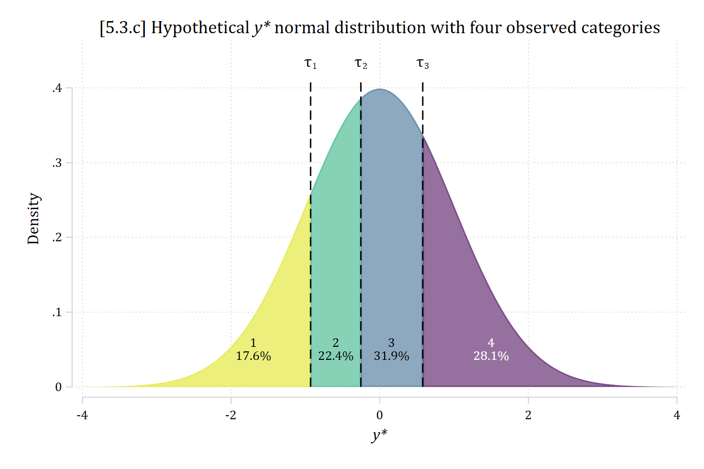
*5.3.c - hypothetical y* split into four ordinal categories
twoway function y=normalden(x), range(-4 -.930) recast(area) color("222 227 24
*.7") || ///
    function y=normalden(x), range(-.930 -.254) recast(area) color("41 175 127
*.7") || ///
    function y=normalden(x), range(-.254 .579) recast(area) color("50 100 142*
.7") || ///
    function y=normalden(x), range(.579 4) recast(area) color("68 1 84*.7") ||
 ///
    pci 0 -.930 .41 -.930 0 -.254 .41 -.254 0 .579 .41 .579, lcolor(black) lpa
ttern(dash) ///
    xtitle("{it:y*}") ytitle("Density") legend(off) xlabel(-4(2)4) ///
    yscale(range(0 .45)) ylabel(0(.1).4) ///
    title("[5.3.c] Hypothetical {it:y*} normal distribution with four observed
 categories") ///
    text(.435 -.930 "{&tau}{sub:1}" .435 -.254 "{&tau}{sub:2}" .435 .579 "{&ta
u}{sub:3}") ///
    text(.05 -1.7 "1" "17.6%" .05 -.59 "2" "22.4%" .05 .16 "3" "31.9%", size(s
mall)) ///
    text(.05 1.5 "4" "28.1%", size(small) color(white))

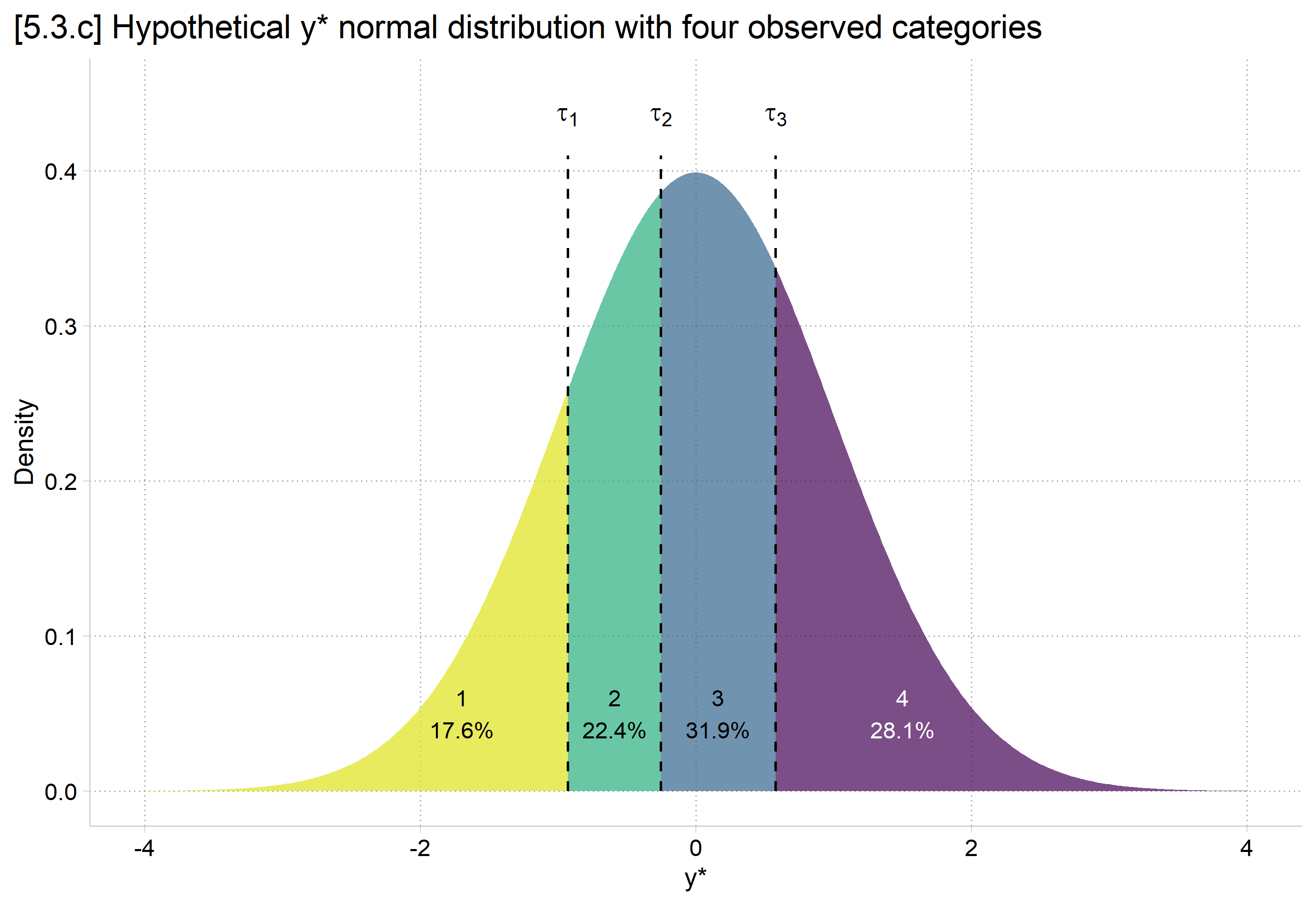
[5.3.c] Standard normal density of a hypothetical y-star split by dashed lines at tau 1 = -0.930, tau 2 = -0.254, and tau 3 = 0.579 into four shaded areas: category 1 (17.6%), 2 (22.4%), 3 (31.9%), and 4 (28.1%).

# 5.3.c - hypothetical y* split into four ordinal categories
cuts <- c(-.930, -.254, .579)
bounds <- c(-4, cuts, 4)
ystar <- bind_rows(lapply(1:4, function(j) {
  data.frame(category = factor(j), x = seq(bounds[j], bounds[j + 1], length.out = 200))
})) |>
  mutate(density = dnorm(x))

ggplot(ystar, aes(x = x, ymin = 0, ymax = density, fill = category)) +
  geom_ribbon(alpha = .7) +
  geom_segment(data = data.frame(x = cuts), aes(x = x, xend = x, y = 0, yend = .41),
    inherit.aes = FALSE, linetype = "dashed") +
  annotate("text", x = cuts, y = .435, label = c("tau[1]", "tau[2]", "tau[3]"), parse = TRUE) +
  annotate("text", x = c(-1.7, -.59, .16, 1.5), y = .05,
    label = c("1\n17.6%", "2\n22.4%", "3\n31.9%", "4\n28.1%"),
    color = c("black", "black", "black", "white"), size = 3.5) +
  scale_fill_manual(values = c("#DEE318", "#29AF7F", "#32648E", "#440154")) +
  scale_x_continuous(breaks = seq(-4, 4, 2)) +
  scale_y_continuous(breaks = seq(0, .4, .1), limits = c(0, .45)) +
  labs(title = "[5.3.c] Hypothetical y* normal distribution with four observed categories",
    x = "y*", y = "Density") +
  theme(legend.position = "none", plot.title.position = "plot")

[5.3.c] Standard normal density of a hypothetical y-star split by dashed lines at tau 1 = -0.930, tau 2 = -0.254, and tau 3 = 0.579 into four shaded areas: category 1 (17.6%), 2 (22.4%), 3 (31.9%), and 4 (28.1%).

Ordinal probit threshold estimates

  • Compare the z-scores above to the estimated thresholds (“cuts” in Stata speak) from ordinal probit:
*Show estimated thresholds (taus) and model average probabilities
oprobit pillokR
Iteration 0:  Log likelihood = -34042.826  
Iteration 1:  Log likelihood = -34042.826  

Ordered probit regression                               Number of obs = 24,993
Log likelihood = -34042.826                             Pseudo R2     = 0.0000

------------------------------------------------------------------------------
     pillokR | Coefficient  Std. err.      z    P>|z|     [95% conf. interval]
-------------+----------------------------------------------------------------
       /cut1 |     -0.930      0.009                        -0.948      -0.912
       /cut2 |     -0.254      0.008                        -0.270      -0.238
       /cut3 |      0.579      0.008                         0.562       0.595
------------------------------------------------------------------------------
# Show estimated thresholds (taus)
probmod <- polr(pillokR ~ 1, data = gss, method = "probit", Hess = TRUE)
summary(probmod)
Call:
polr(formula = pillokR ~ 1, data = gss, Hess = TRUE, method = "probit")

No coefficients

Intercepts:
                  Value    Std. Error t value 
StrDisag|Disagree  -0.9299   0.0093   -99.8995
Disagree|Agree     -0.2539   0.0080   -31.6514
Agree|StrAgree      0.5787   0.0084    68.6503

Residual Deviance: 68085.65 
AIC: 68091.65 
  • Thus, the metric of y* is determined partially by the distribution of the dependent variable
    • Do you find this a substantively meaningful way to decide on the category spacing of the latent continuum y*?
    • Can you think of a better alternative?

The good and the bad of the thresholds

  • The reason for setting the spacing of the thresholds based on the cumulative distribution is clear: it allows the model to uncover probabilities whose distribution match those of the observed proportions in the data (compare to the pillokR frequency table above)
margins
warning: prediction constant over observations.

Predictive margins                                      Number of obs = 24,993
Model VCE: OIM

1._predict: Pr(pillokR==1), predict(pr outcome(1))
2._predict: Pr(pillokR==2), predict(pr outcome(2))
3._predict: Pr(pillokR==3), predict(pr outcome(3))
4._predict: Pr(pillokR==4), predict(pr outcome(4))

------------------------------------------------------------------------------
             |            Delta-method
             |     Margin   std. err.      z    P>|z|     [95% conf. interval]
-------------+----------------------------------------------------------------
    _predict |
          1  |      0.176      0.002   73.116   0.000        0.171       0.181
          2  |      0.224      0.003   84.836   0.000        0.218       0.229
          3  |      0.319      0.003  108.153   0.000        0.313       0.325
          4  |      0.281      0.003   98.930   0.000        0.276       0.287
------------------------------------------------------------------------------
avg_predictions(probmod)

    Group Estimate Std. Error     z Pr(>|z|)   S 2.5 % 97.5 %
 StrDisag    0.176    0.00241  73.1   <0.001 Inf 0.171  0.181
 Disagree    0.224    0.00264  84.8   <0.001 Inf 0.218  0.229
 Agree       0.319    0.00295 108.2   <0.001 Inf 0.313  0.325
 StrAgree    0.281    0.00284  98.9   <0.001 Inf 0.276  0.287

Type: probs
Back to top