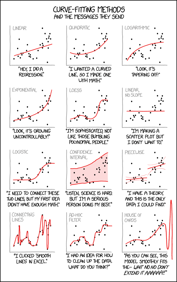
2.6 Assessing and Modeling Complex Nonlinearities for Independent Variables
- Thus far, we have only covered the relatively simple case of adding a squared term for a continuous IV. However, there are many other ways to assess and model nonlinearities in regression models
- Note it is not always best to use the most complicated solution
- Indeed, some of these more flexible methods are helpful for assessing when you are OK using the simpler solution
- However, it is generally impossible to know whether the simpler solution is OK unless you have also tried the more complicated solution
- A footnote stating “I tried it the more sophisticated way and found basically the same exact result as the easier way” can be very reassuring to reviewers; in that case, present the easier way in the main text
- All else equal, simplicity is a virtue. However, simplicity is not a valid justification for inaccurately modeling your data*
*E.g., Would you be comfortable writing a paper with the occupational prestige, gender, and age data above that did not include age2? That did not include interactions between age and gender?
Scatterplots
- For bivariate relationships, scatterplots can be helpful
use "https://tdmize.github.io/data/data/regjob3", clear(Long's data on academic jobs of biochemists \ 2009-03-13)sort phd
twoway scatter job phd, jitter(3) ///
title("[2.6.a] Job Prestige and Prestige of PhD Program")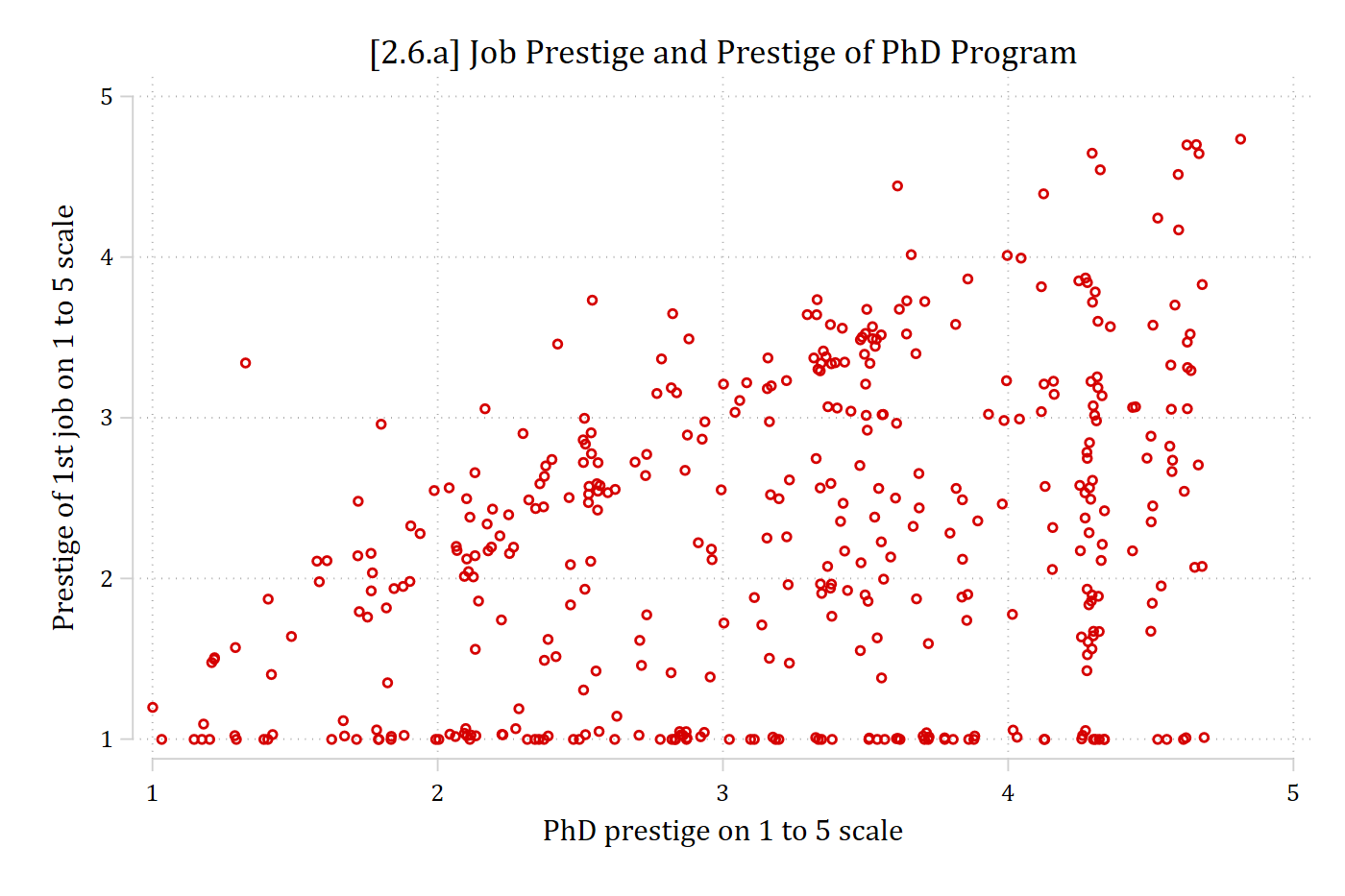
twoway scatter job phd if fem == 0, jitter(3) || ///
    scatter job phd if fem == 1, jitter(3) || , ///
    title("[2.6.b] Job Prestige and Prestige of PhD Program") ///
    legend(order(1 "Men" 2 "Women"))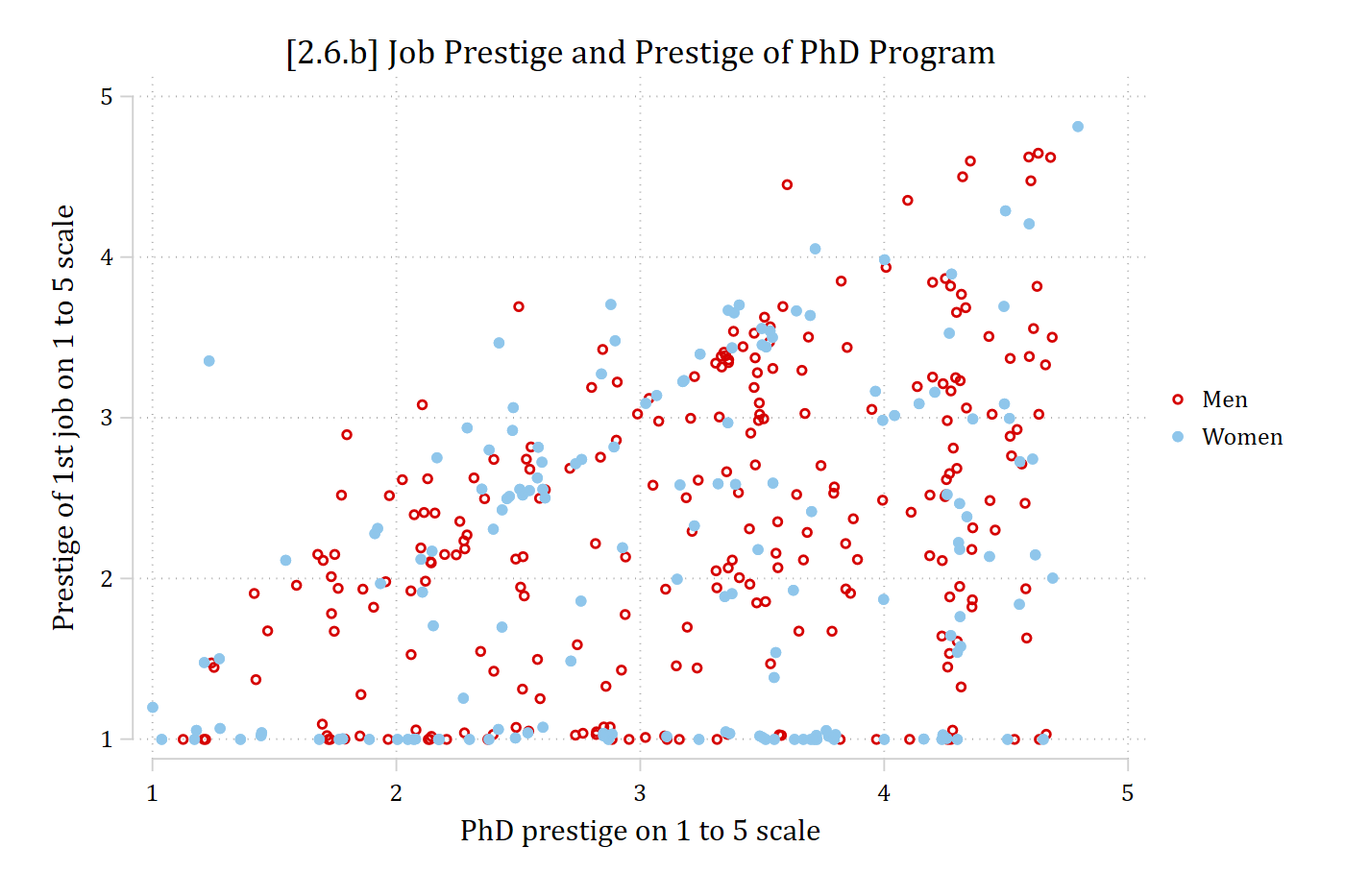
LOWESS: locally weighted scatterplot smoothing
- Lowess performs “local” regressions sequentially across subsets of your data, showing how one continuous IV relates to a DV across the range of your data
- This is primarily an exploratory technique—you can plot the smoothed regression line but you do not get parameter estimates or tests of statistical significance
- It can be a helpful way to quickly assess nonlinearity and often suggests possible parametric modeling solutions for the nonlinearity (e.g., need both age and age2 in model)
- Since a lowess plot is non-parametric it does not constrain the shape of the relationship between an IV and the DV in any way
- A bandwidth can be specified to determine just how local you want the lowess to calculate the regression estimate
- A bandwidth of 0.4 means you want the 40% of the data closest to a given point used to calculate the regression line for that point (data points closer to the middle of the bandwidth are given more weight)
- Smaller bandwidths will let you find more nonlinearities but are more susceptible to outliers and other quirks of your data
lowess job phd, bwidth(0.8)
lowess job phd, bwidth(0.2)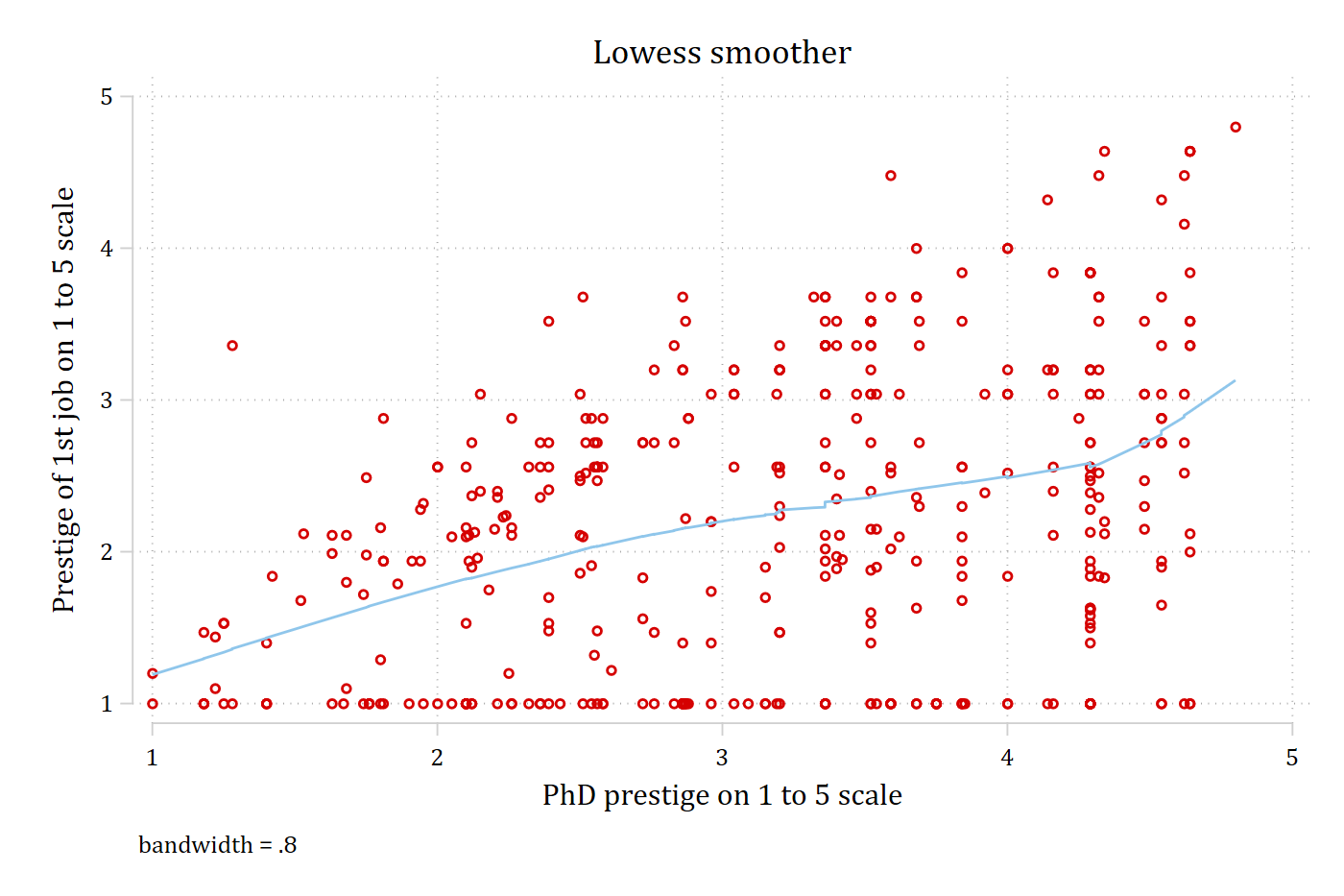
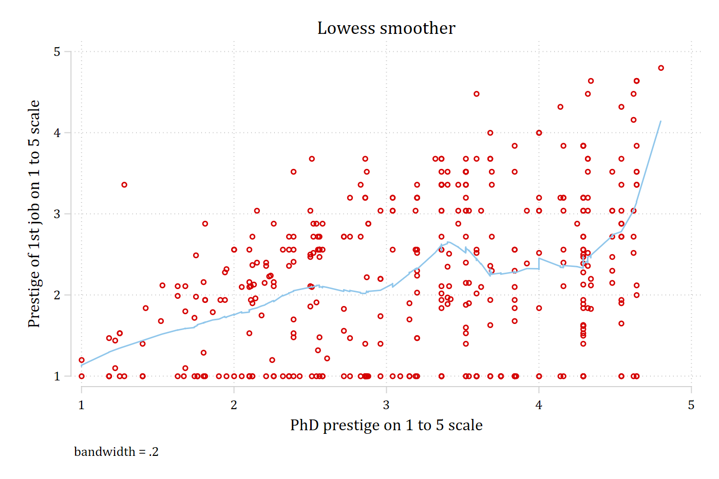
- Bandwidth of 0.8 too wide to be informative (left panel above); mostly same as a linear fit
- Bandwidth of 0.2 is too small: it picks up on too many quirks of the data that we don’t want to model (right panel above)
- Sharp jumps in the line often suggest a too-small bandwidth
use "https://tdmize.github.io/data/data/cda_gss", clear(cda_gss.dta | GSS 1972-2021 CDA - Categorical Data Analysis | date created 202
> 3)replace freespchSS = freespchSS * 100(37,790 real changes made)hist freespchSS, percent ///
title("[2.6.g] Distribution of support for free speech scale") ///
subtitle("0% = restrict free speech in all cases; 100% = support free spee
ch in all cases")(bin=46, start=0, width=2.173913)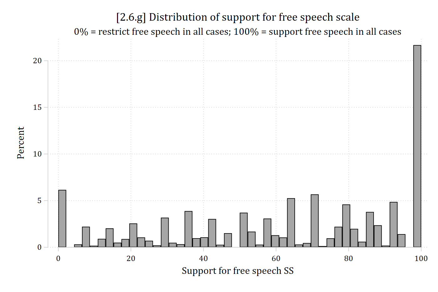
lowess freespchSS edyrs, bwidth(.4) jitter(3) xlab(0(2)20) gen(lowpr) ///
    title("[2.6.h] Relationship between support for free speech and education"
) ///
    subtitle("With lowess smoothed trend line") ytitle("Support for free speec
h")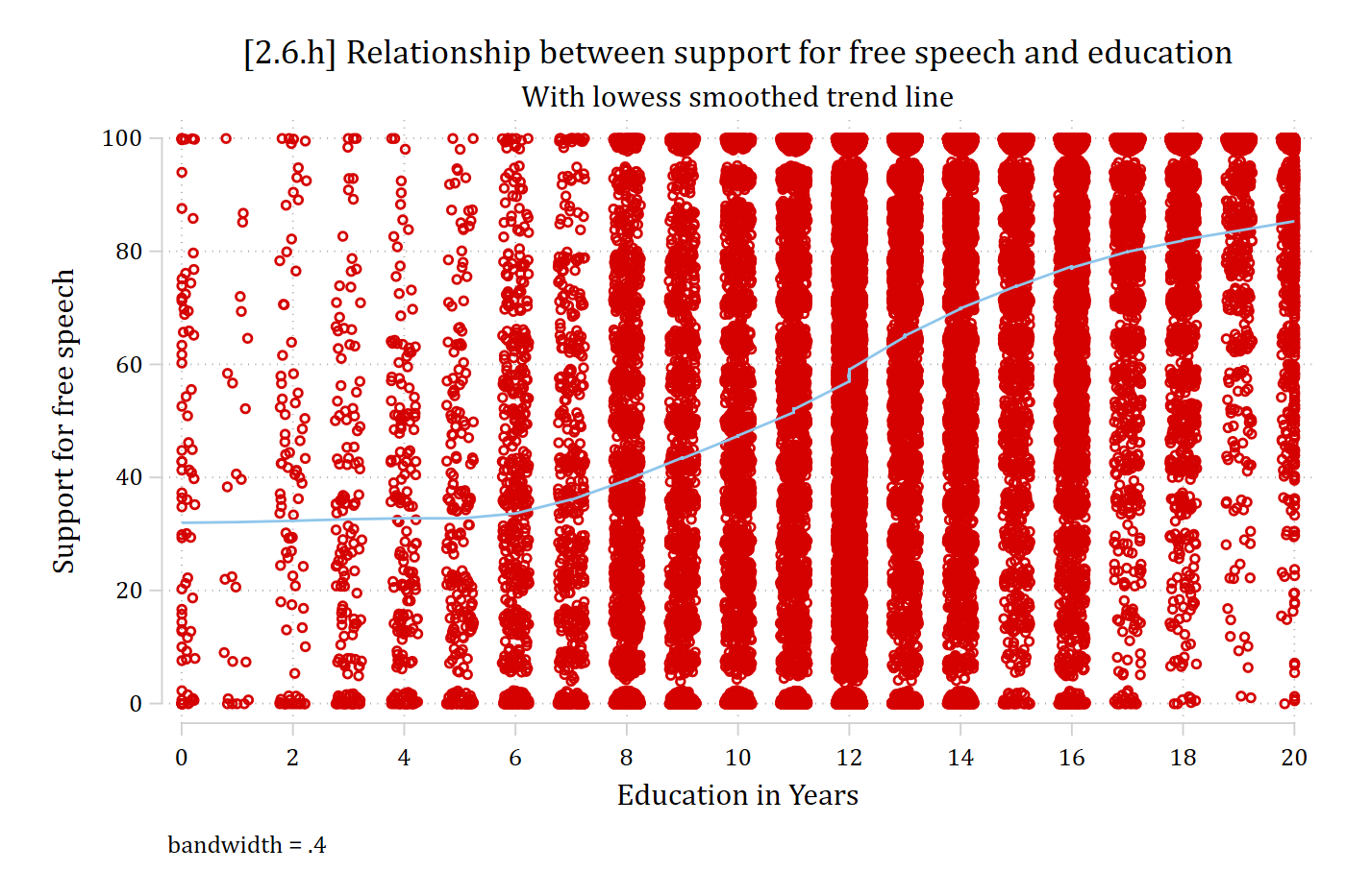
reg freespchSS c.edyrs##c.edyrs##c.edyrs Source | SS df MS Number of obs = 40,152
-------------+---------------------------------- F(3, 40148) = 2973.88
Model | 7555022.18 3 2518340.73 Prob > F = 0.0000
Residual | 33998175.3 40,148 846.821144 R-squared = 0.1818
-------------+---------------------------------- Adj R-squared = 0.1818
Total | 41553197.5 40,151 1034.9231 Root MSE = 29.1
------------------------------------------------------------------------------
freespchSS | Coefficient Std. err. t P>|t| [95% conf. interval]
-------------+----------------------------------------------------------------
edyrs | -8.298 0.596 -13.934 0.000 -9.465 -7.131
|
c.edyrs#|
c.edyrs | 1.186 0.054 21.792 0.000 1.080 1.293
|
c.edyrs#|
c.edyrs#|
c.edyrs | -0.034 0.002 -21.703 0.000 -0.037 -0.031
|
_cons | 45.488 2.107 21.587 0.000 41.358 49.618
------------------------------------------------------------------------------All three edyrs coefficients are highly significant, suggesting that including them improves model fit (but note this is a very large sample)
margins, at(edyrs=(0(1)20))Adjusted predictions Number of obs = 40,152
Model VCE: OLS
Expression: Linear prediction, predict()
1._at: edyrs = 0
2._at: edyrs = 1
3._at: edyrs = 2
4._at: edyrs = 3
5._at: edyrs = 4
6._at: edyrs = 5
7._at: edyrs = 6
8._at: edyrs = 7
9._at: edyrs = 8
10._at: edyrs = 9
11._at: edyrs = 10
12._at: edyrs = 11
13._at: edyrs = 12
14._at: edyrs = 13
15._at: edyrs = 14
16._at: edyrs = 15
17._at: edyrs = 16
18._at: edyrs = 17
19._at: edyrs = 18
20._at: edyrs = 19
21._at: edyrs = 20
------------------------------------------------------------------------------
| Delta-method
| Margin std. err. t P>|t| [95% conf. interval]
-------------+----------------------------------------------------------------
_at |
1 | 45.488 2.107 21.587 0.000 41.358 49.618
2 | 38.342 1.605 23.889 0.000 35.196 41.488
3 | 33.366 1.207 27.635 0.000 31.000 35.733
4 | 30.358 0.906 33.495 0.000 28.582 32.135
5 | 29.114 0.692 42.075 0.000 27.758 30.470
6 | 29.431 0.550 53.537 0.000 28.354 30.509
7 | 31.108 0.459 67.802 0.000 30.208 32.007
8 | 33.940 0.396 85.750 0.000 33.164 34.716
9 | 37.725 0.343 110.090 0.000 37.054 38.397
10 | 42.261 0.291 145.377 0.000 41.691 42.831
11 | 47.344 0.240 197.300 0.000 46.874 47.814
12 | 52.772 0.198 266.998 0.000 52.384 53.159
13 | 58.342 0.175 333.527 0.000 57.999 58.684
14 | 63.851 0.177 360.987 0.000 63.504 64.197
15 | 69.096 0.194 355.900 0.000 68.715 69.476
16 | 73.874 0.213 346.047 0.000 73.456 74.293
17 | 77.984 0.231 337.577 0.000 77.531 78.436
18 | 81.221 0.260 312.841 0.000 80.712 81.730
19 | 83.383 0.330 252.667 0.000 82.736 84.030
20 | 84.268 0.472 178.569 0.000 83.343 85.193
21 | 83.672 0.698 119.818 0.000 82.303 85.041
------------------------------------------------------------------------------marginsplot, plotop(msymbol(none)) recastci(rline) ciopt(lpat(dash) lcol(*.4))
///
ylab(0(10)100) ytitle("free speech support") ///
title("[2.6.i] Predicted support for free speech by education in years") /
//
addplot(connected lowpr edyrs, sort msymbol(none) lcol(eltblue)) ///
legend(order(2 "edyrs^3" 3 "lowess"))Variables that uniquely identify margins: edyrs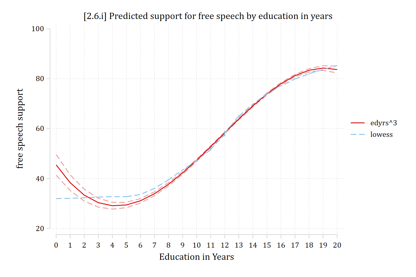
Splines
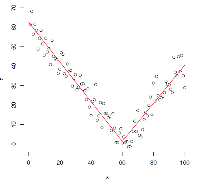
- An alternative to polynomial IVs is splines which allow for an abrupt change in the prediction line
- Essentially, estimate a coefficient for each piece of the relationship separately allowing entirely different slopes
- For an overview of splines, see Appendix 2C
- For details on coding splines in Stata, see Appendix A2.8
Binned scatterplots
- Scatterplot methods are less useful when you have lots of data
- Graphs become impossible to read (but could plot random subsample) and lowess becomes computationally intensive
- A binned scatterplot is a useful tool for these and other cases (Stepner 2014)
- “bin” the x variable into groups (e.g., 20 age groups) and then calculate the mean of the y variable for each bin
Table 1: Descriptive Statistics for 21 waves of longitudinal data of Australians (N2 = 29,186; N1 = 242,933)
| Mean | SD | Min. | Max. | |
|---|---|---|---|---|
| Physical Health Scale | 77.37 | 21.38 | 0.00 | 100.00 |
| Mental Health Scale | 72.23 | 19.13 | 0.00 | 100.00 |
| Role Count | 4.15 | 1.33 | 0.00 | 8.00 |
| Age | 46.57 | 17.93 | 18.00 | 101.00 |
The rest of this page uses restricted-access data (the HILDA survey), so the data file is not available to download.
use "RaRc-03-analysis", clear(RaRc | Analysis data)gen roles = oroles + vroles
lab var roles "Number of social roles"
scatter PHscale age, jitter(3) ///
title("[2.6.j] HILDA data: N = 242,933")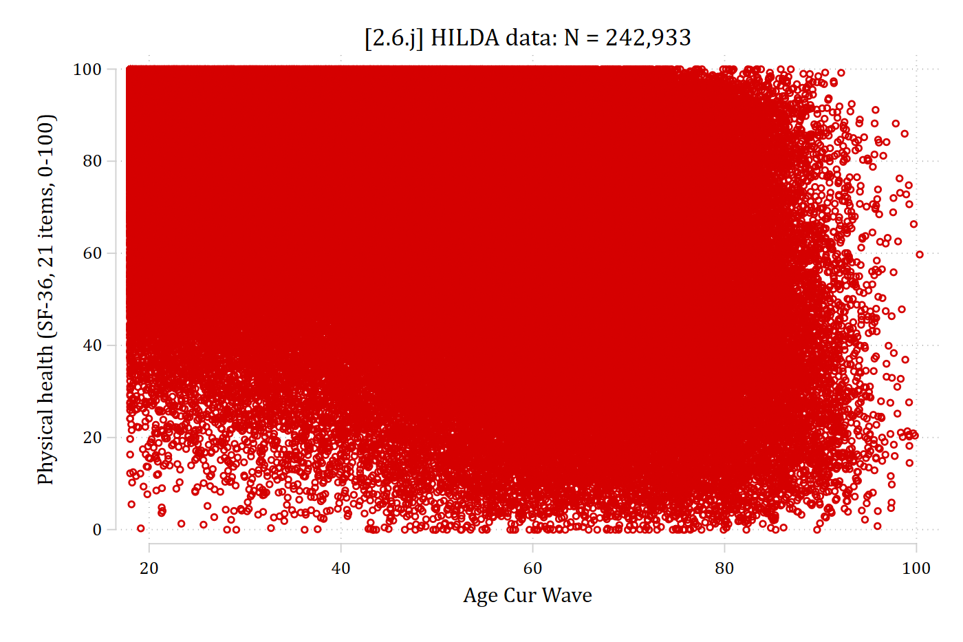
binscatter PHscale age, ///
    title("[2.6.k] Binned scatterplot for physical health by age") ///
    ytitle("Physical health scale") line(none)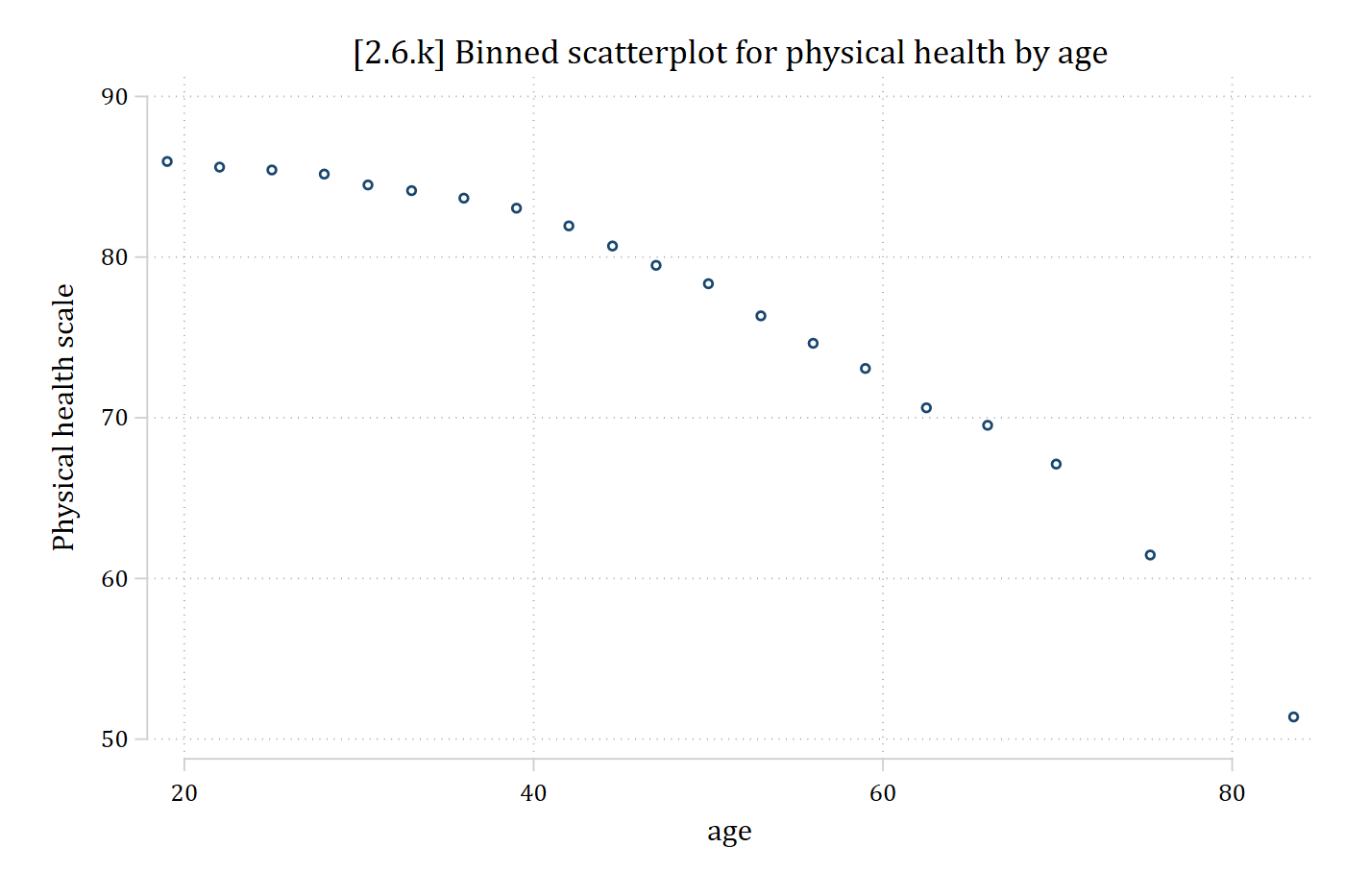
binscatterhist PHscale age, line(qfit) ///
    title("[2.6.l] Binned scatterplot for physical health by age") ///
    subtitle("Including a quadratic line fit") ///
    ytitle("Physical health scale")
(242,933 real changes made)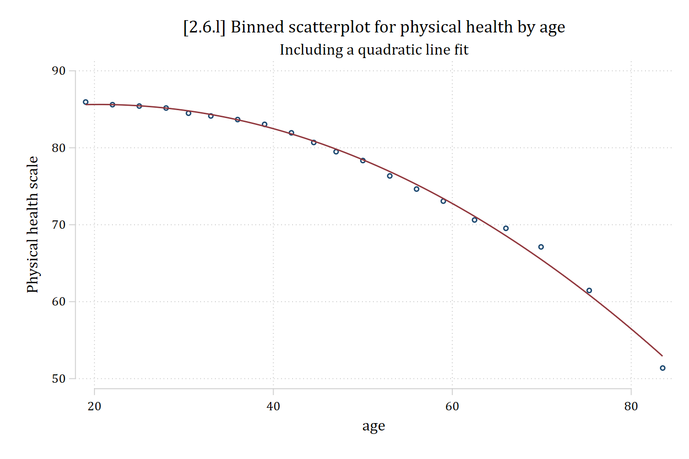
Treating a continuous or ordinal IV as nominal
- A limitation of the methods covered above is they only examine bivariate relationships*; often, we want to know conditional relationships after controlling for other variables
- Also limited to relatively simple regressions; e.g., cannot examine multilevel or fixed effect models
- An elegantly simple but remarkably flexible way to examine the functional form of a continuous IV is to treat it as a nominal variable in your regression model
- E.g., Omit 0 as reference category for social roles; add coefficients for 1, 2, 3, 4…8 roles
- For IVs with lots of values, you can “coarsen” or “bin” them first
- E.g., Create age categories of 20 – 30, 31 – 40, 41 – 50, etc.
- Can use this technique for almost any regression model and almost any DV type
- For this technique, you want to go straight to graphs rather than worrying about the coefficient estimates
*Can use lowess with control variables with the mlowess command but it is limited
reg MHscale i.roles ///
    i.male c.hhincome c.age i.educ i.wave, cluster(ID)
Linear regression Number of obs = 242,933
F(35, 29185) = 127.82
Prob > F = 0.0000
R-squared = 0.0839
Root MSE = 18.31
(Std. err. adjusted for 29,186 clusters in ID)
------------------------------------------------------------------------------
| Robust
MHscale | Coefficient std. err. t P>|t| [95% conf. interval]
-------------+----------------------------------------------------------------
roles |
1 | 2.911 1.594 1.826 0.068 -0.214 6.037
2 | 6.972 1.645 4.238 0.000 3.747 10.196
3 | 12.762 1.647 7.746 0.000 9.532 15.991
4 | 16.818 1.647 10.210 0.000 13.589 20.046
5 | 19.302 1.649 11.708 0.000 16.070 22.533
6 | 20.382 1.653 12.327 0.000 17.141 23.622
7 | 21.102 1.669 12.646 0.000 17.831 24.372
8 | 18.821 2.467 7.630 0.000 13.986 23.656
|
male |
Yes | 3.007 0.206 14.616 0.000 2.603 3.410
hhincome | 0.233 0.012 20.059 0.000 0.210 0.255
age | 0.097 0.006 16.733 0.000 0.086 0.108
|
educ |
HS | 2.026 0.342 5.933 0.000 1.357 2.696
SomeCol | 0.793 0.290 2.734 0.006 0.225 1.362
College | 2.019 0.327 6.168 0.000 1.377 2.660
Graduate | 1.932 0.356 5.431 0.000 1.235 2.629
|
wave |
3 | -0.392 0.182 -2.161 0.031 -0.748 -0.036
4 | -0.463 0.195 -2.373 0.018 -0.845 -0.081
5 | -0.470 0.194 -2.421 0.015 -0.851 -0.090
6 | -0.211 0.204 -1.033 0.302 -0.612 0.190
7 | -0.451 0.211 -2.133 0.033 -0.865 -0.037
8 | -0.687 0.216 -3.184 0.001 -1.110 -0.264
9 | -0.436 0.217 -2.008 0.045 -0.861 -0.010
10 | -1.127 0.217 -5.202 0.000 -1.551 -0.702
11 | -0.939 0.209 -4.497 0.000 -1.348 -0.530
12 | -0.764 0.213 -3.587 0.000 -1.182 -0.347
13 | -1.030 0.217 -4.746 0.000 -1.456 -0.605
14 | -1.763 0.222 -7.946 0.000 -2.198 -1.328
15 | -2.305 0.223 -10.334 0.000 -2.743 -1.868
16 | -2.084 0.221 -9.437 0.000 -2.517 -1.652
17 | -2.793 0.226 -12.354 0.000 -3.236 -2.350
18 | -3.135 0.229 -13.674 0.000 -3.584 -2.685
19 | -3.827 0.233 -16.407 0.000 -4.284 -3.370
20 | -5.193 0.236 -22.023 0.000 -5.655 -4.731
21 | -5.701 0.241 -23.625 0.000 -6.174 -5.228
22 | -5.931 0.246 -24.148 0.000 -6.412 -5.449
|
_cons | 49.168 1.687 29.139 0.000 45.861 52.476
------------------------------------------------------------------------------qui margins, at(roles=(0(1)8)) saving(m_cat, replace)
marginsplot, ///
title("[2.6.m] Predictions from Categorical Form of Social Roles", size(me
dium)) ///
ytitle("Mental Health Scale") xtitle("Number of Social Roles")Variables that uniquely identify margins: roles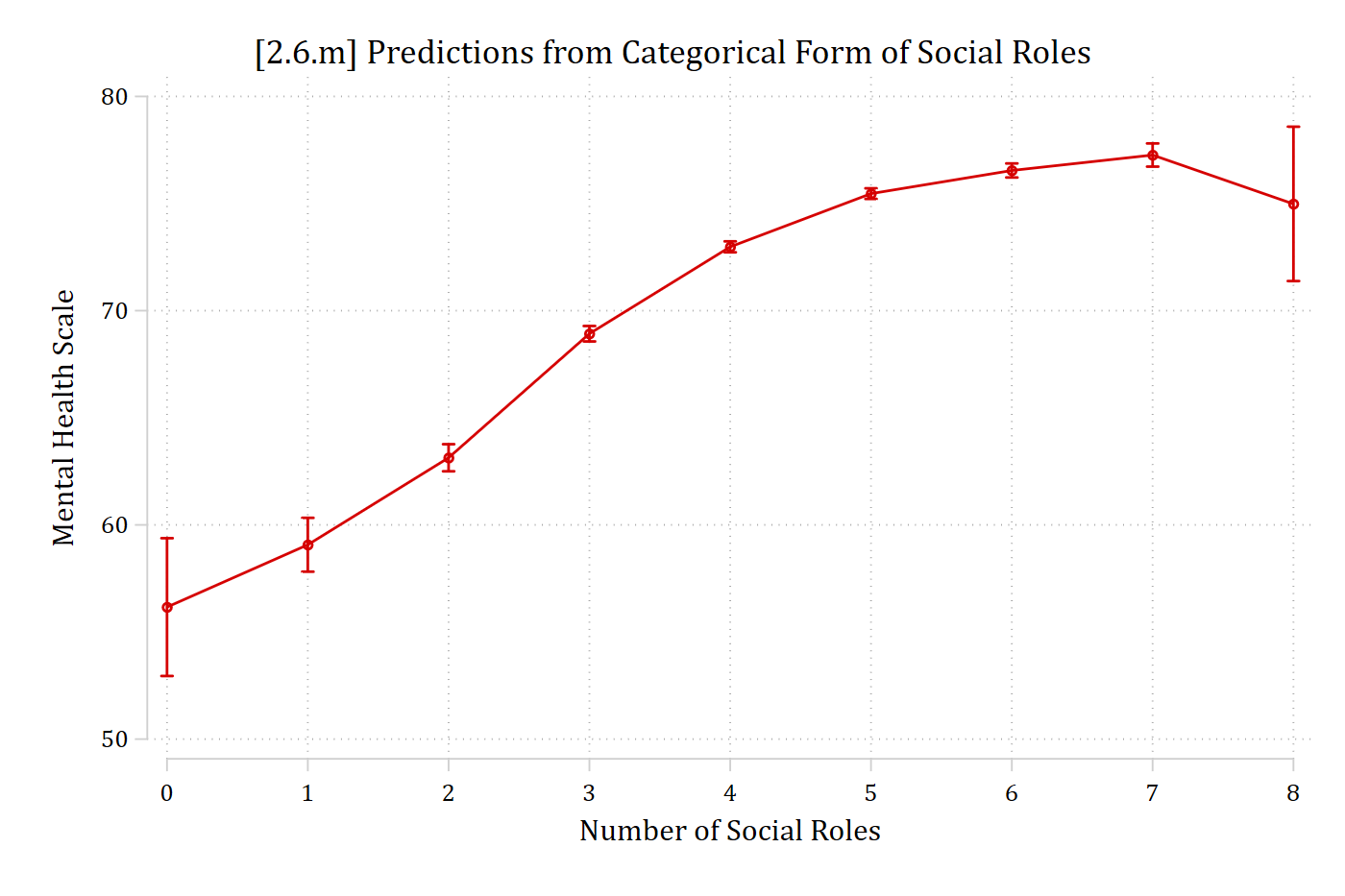
Note, despite this pattern, there is no monotonic restriction on the functional form
- Can we model this relationship parametrically?
reg MHscale c.roles##c.roles ///
    i.male c.hhincome c.age i.educ i.wave, cluster(ID)
Linear regression Number of obs = 242,933
F(29, 29185) = 151.90
Prob > F = 0.0000
R-squared = 0.0833
Root MSE = 18.316
(Std. err. adjusted for 29,186 clusters in ID)
------------------------------------------------------------------------------
| Robust
MHscale | Coefficient std. err. t P>|t| [95% conf. interval]
-------------+----------------------------------------------------------------
roles | 7.668 0.324 23.697 0.000 7.034 8.303
|
c.roles#|
c.roles | -0.561 0.035 -15.982 0.000 -0.630 -0.492
|
male |
Yes | 3.013 0.206 14.638 0.000 2.610 3.417
hhincome | 0.234 0.012 20.110 0.000 0.211 0.256
age | 0.096 0.006 16.474 0.000 0.084 0.107
|
educ |
HS | 2.032 0.342 5.943 0.000 1.362 2.702
SomeCol | 0.814 0.290 2.803 0.005 0.245 1.383
College | 2.039 0.328 6.221 0.000 1.397 2.682
Graduate | 1.957 0.356 5.500 0.000 1.260 2.655
|
wave |
3 | -0.397 0.181 -2.188 0.029 -0.752 -0.041
4 | -0.460 0.195 -2.357 0.018 -0.842 -0.077
5 | -0.463 0.194 -2.384 0.017 -0.844 -0.082
6 | -0.206 0.204 -1.010 0.313 -0.607 0.194
7 | -0.452 0.211 -2.137 0.033 -0.866 -0.037
8 | -0.685 0.216 -3.174 0.002 -1.107 -0.262
9 | -0.431 0.217 -1.986 0.047 -0.856 -0.006
10 | -1.129 0.217 -5.211 0.000 -1.553 -0.704
11 | -0.937 0.209 -4.486 0.000 -1.346 -0.527
12 | -0.764 0.213 -3.586 0.000 -1.182 -0.347
13 | -1.031 0.217 -4.747 0.000 -1.456 -0.605
14 | -1.763 0.222 -7.942 0.000 -2.198 -1.328
15 | -2.307 0.223 -10.335 0.000 -2.744 -1.869
16 | -2.088 0.221 -9.447 0.000 -2.521 -1.655
17 | -2.790 0.226 -12.331 0.000 -3.233 -2.346
18 | -3.138 0.229 -13.684 0.000 -3.587 -2.688
19 | -3.828 0.233 -16.400 0.000 -4.285 -3.371
20 | -5.202 0.236 -22.048 0.000 -5.665 -4.740
21 | -5.714 0.242 -23.658 0.000 -6.187 -5.241
22 | -5.940 0.246 -24.161 0.000 -6.421 -5.458
|
_cons | 44.100 0.833 52.972 0.000 42.468 45.731
------------------------------------------------------------------------------qui margins, at(roles=(0(.25)8))
marginsplot, plotopt(lcol(eltblue) msym(none)) ///
recastci(rline) ciopts(lpat(dash) col(eltblue*.5)) ///
title("[2.6.n] Predictions from Quadratic Form of Social Roles", size(medi
um)) ///
ytitle("Mental Health Scale") xtitle("Number of Social Roles")Variables that uniquely identify margins: roles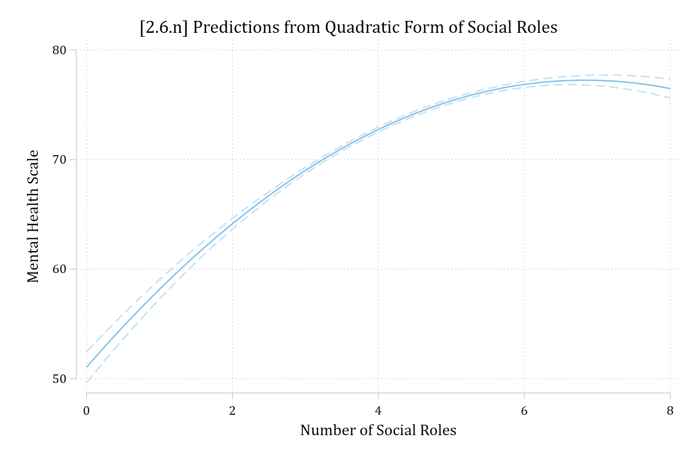
*Note: The addition of the polynomial roles2 allows for a change in the slope
qui margins, at(roles=(0(1)8)) saving(m_sq, replace)
combomarginsplot m_cat m_sq, ///
    labels("Categorical Model" "Quadratic Model") ///
    title("[2.6.o] Comparison of Predictions for Various Functional Forms of R
oles", size(medium)) ///
    ytitle("Mental Health Scale") xtitle("Number of Social Roles")
Variables that uniquely identify margins: roles _filenumber
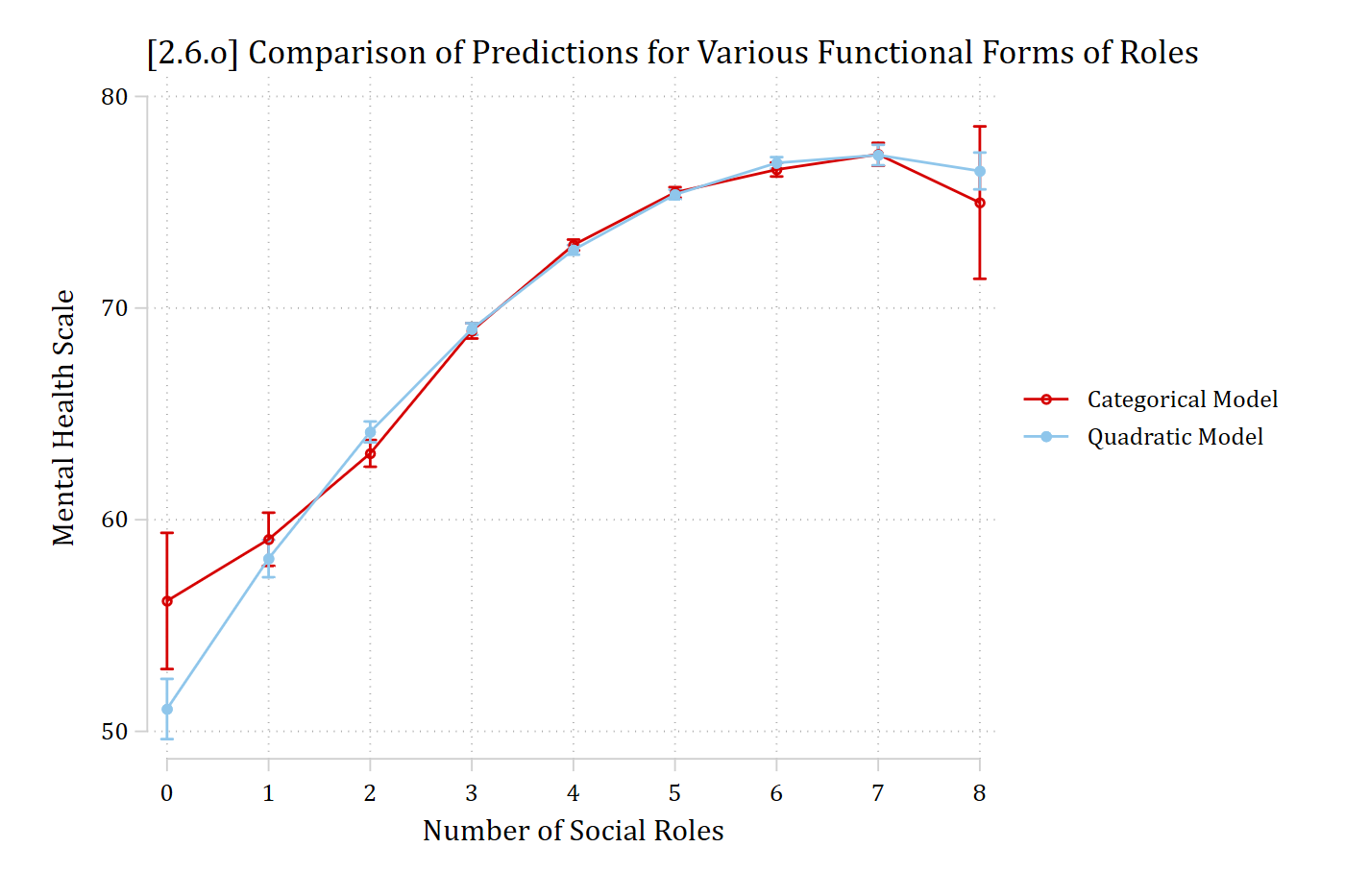
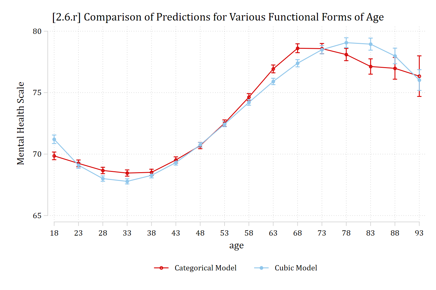
The simple addition of roles2 does a remarkably good job here
xtset ID wavePanel variable: ID (unbalanced)
Time variable: wave, 2 to 22, but with gaps
Delta: 1 unitsum age Variable | Obs Mean Std. dev. Min Max
-------------+---------------------------------------------------------
age | 242,933 46.56807 17.92905 18 101egen ageC = cut(age), at(18(5)110)
fre ageCageC
-----------------------------------------------------------
| Freq. Percent Valid Cum.
--------------+--------------------------------------------
Valid 18 | 21275 8.76 8.76 8.76
23 | 22067 9.08 9.08 17.84
28 | 22324 9.19 9.19 27.03
33 | 21810 8.98 8.98 36.01
38 | 21462 8.83 8.83 44.84
43 | 21839 8.99 8.99 53.83
48 | 21236 8.74 8.74 62.57
53 | 20185 8.31 8.31 70.88
58 | 18351 7.55 7.55 78.44
63 | 16253 6.69 6.69 85.13
68 | 13613 5.60 5.60 90.73
73 | 10290 4.24 4.24 94.97
78 | 6829 2.81 2.81 97.78
83 | 3665 1.51 1.51 99.29
88 | 1407 0.58 0.58 99.87
93 | 298 0.12 0.12 99.99
98 | 29 0.01 0.01 100.00
Total | 242933 100.00 100.00
-----------------------------------------------------------recode ageC 93/110 = 93(29 changes made to ageC)* Person means of the role counts and their squares
bysort ID: egen orolesM = mean(oroles)
bysort ID: egen oroles2M = mean(oroles^2)
bysort ID: egen vrolesM = mean(vroles)
bysort ID: egen vroles2M = mean(vroles^2)
xtreg MHscale i.ageC ///
c.oroles##c.oroles c.vroles##c.vroles ///
c.orolesM c.oroles2M c.vrolesM c.vroles2M ///
physfunc ib3.educ c.hhincome i.wave, reRandom-effects GLS regression Number of obs = 242,933
Group variable: ID Number of groups = 29,186
R-squared: Obs per group:
Within = 0.0967 min = 1
Between = 0.2670 avg = 8.3
Overall = 0.2424 max = 21
Wald chi2(49) = 33654.68
corr(u_i, X) = 0 (assumed) Prob > chi2 = 0.0000
------------------------------------------------------------------------------
MHscale | Coefficient Std. err. z P>|z| [95% conf. interval]
-------------+----------------------------------------------------------------
ageC |
23 | -0.611 0.137 -4.452 0.000 -0.880 -0.342
28 | -1.189 0.155 -7.688 0.000 -1.492 -0.886
33 | -1.397 0.169 -8.275 0.000 -1.728 -1.066
38 | -1.339 0.181 -7.392 0.000 -1.695 -0.984
43 | -0.335 0.190 -1.764 0.078 -0.707 0.037
48 | 0.840 0.199 4.228 0.000 0.450 1.229
53 | 2.658 0.208 12.763 0.000 2.250 3.066
58 | 4.779 0.220 21.734 0.000 4.348 5.210
63 | 7.076 0.235 30.139 0.000 6.616 7.536
68 | 8.758 0.254 34.468 0.000 8.260 9.256
73 | 8.729 0.279 31.237 0.000 8.181 9.276
78 | 8.245 0.315 26.191 0.000 7.628 8.862
83 | 7.272 0.373 19.513 0.000 6.542 8.003
88 | 7.123 0.494 14.420 0.000 6.155 8.091
93 | 6.487 0.868 7.474 0.000 4.786 8.188
|
oroles | 1.557 0.180 8.643 0.000 1.204 1.909
|
c.oroles#|
c.oroles | -0.107 0.032 -3.331 0.001 -0.171 -0.044
|
vroles | 1.997 0.097 20.626 0.000 1.807 2.187
|
c.vroles#|
c.vroles | -0.282 0.028 -9.992 0.000 -0.338 -0.227
|
orolesM | -0.779 0.476 -1.634 0.102 -1.712 0.155
oroles2M | 0.623 0.091 6.812 0.000 0.444 0.802
vrolesM | 6.535 0.411 15.907 0.000 5.730 7.340
vroles2M | -1.267 0.124 -10.205 0.000 -1.510 -1.024
physfunc | 0.251 0.002 145.202 0.000 0.247 0.254
|
educ |
No HS | -0.534 0.165 -3.237 0.001 -0.857 -0.211
HS | -0.004 0.167 -0.025 0.980 -0.330 0.322
College | 0.527 0.182 2.895 0.004 0.170 0.884
Graduate | 0.624 0.213 2.931 0.003 0.207 1.042
|
hhincome | 0.065 0.006 11.704 0.000 0.054 0.076
|
wave |
3 | -0.305 0.171 -1.785 0.074 -0.639 0.030
4 | -0.564 0.173 -3.259 0.001 -0.903 -0.225
5 | -0.553 0.172 -3.225 0.001 -0.890 -0.217
6 | -0.497 0.175 -2.836 0.005 -0.840 -0.153
7 | -0.649 0.177 -3.672 0.000 -0.996 -0.303
8 | -1.116 0.179 -6.234 0.000 -1.467 -0.765
9 | -0.739 0.178 -4.143 0.000 -1.088 -0.389
10 | -1.410 0.176 -8.009 0.000 -1.755 -1.065
11 | -1.266 0.168 -7.523 0.000 -1.596 -0.936
12 | -1.215 0.169 -7.174 0.000 -1.547 -0.883
13 | -1.368 0.170 -8.025 0.000 -1.702 -1.034
14 | -2.116 0.171 -12.341 0.000 -2.452 -1.780
15 | -2.728 0.173 -15.749 0.000 -3.067 -2.388
16 | -2.645 0.173 -15.333 0.000 -2.983 -2.307
17 | -3.092 0.175 -17.699 0.000 -3.434 -2.749
18 | -3.402 0.177 -19.202 0.000 -3.749 -3.055
19 | -4.122 0.178 -23.133 0.000 -4.472 -3.773
20 | -5.855 0.180 -32.515 0.000 -6.208 -5.502
21 | -6.376 0.183 -34.913 0.000 -6.733 -6.018
22 | -6.139 0.187 -32.908 0.000 -6.504 -5.773
|
_cons | 36.673 0.637 57.539 0.000 35.424 37.922
-------------+----------------------------------------------------------------
sigma_u | 12.601915
sigma_e | 11.652285
rho | .53909328 (fraction of variance due to u_i)
------------------------------------------------------------------------------margins ageCPredictive margins Number of obs = 242,933
Model VCE: Conventional
Expression: Linear prediction, predict()
------------------------------------------------------------------------------
| Delta-method
| Margin std. err. z P>|z| [95% conf. interval]
-------------+----------------------------------------------------------------
ageC |
18 | 69.856 0.159 438.994 0.000 69.544 70.168
23 | 69.245 0.140 493.619 0.000 68.970 69.520
28 | 68.667 0.133 517.839 0.000 68.407 68.927
33 | 68.459 0.130 527.367 0.000 68.204 68.713
38 | 68.516 0.129 529.553 0.000 68.263 68.770
43 | 69.521 0.129 539.703 0.000 69.268 69.773
48 | 70.696 0.131 539.145 0.000 70.439 70.953
53 | 72.514 0.137 530.496 0.000 72.246 72.781
58 | 74.634 0.147 508.523 0.000 74.347 74.922
63 | 76.932 0.163 472.842 0.000 76.613 77.251
68 | 78.614 0.184 426.773 0.000 78.253 78.975
73 | 78.584 0.213 369.570 0.000 78.168 79.001
78 | 78.101 0.253 308.908 0.000 77.605 78.596
83 | 77.128 0.318 242.255 0.000 76.504 77.752
88 | 76.979 0.451 170.529 0.000 76.094 77.864
93 | 76.342 0.843 90.591 0.000 74.691 77.994
------------------------------------------------------------------------------marginsplot, recast(scatter) ///
title("[2.6.p] Psychological well-being across ages (binned)", size(medlar
ge)) ///
subtitle("Fixed effects model with controls") ///
xtitle("Age bins in 5 year increments") ytitle("Mental health")Variables that uniquely identify margins: ageC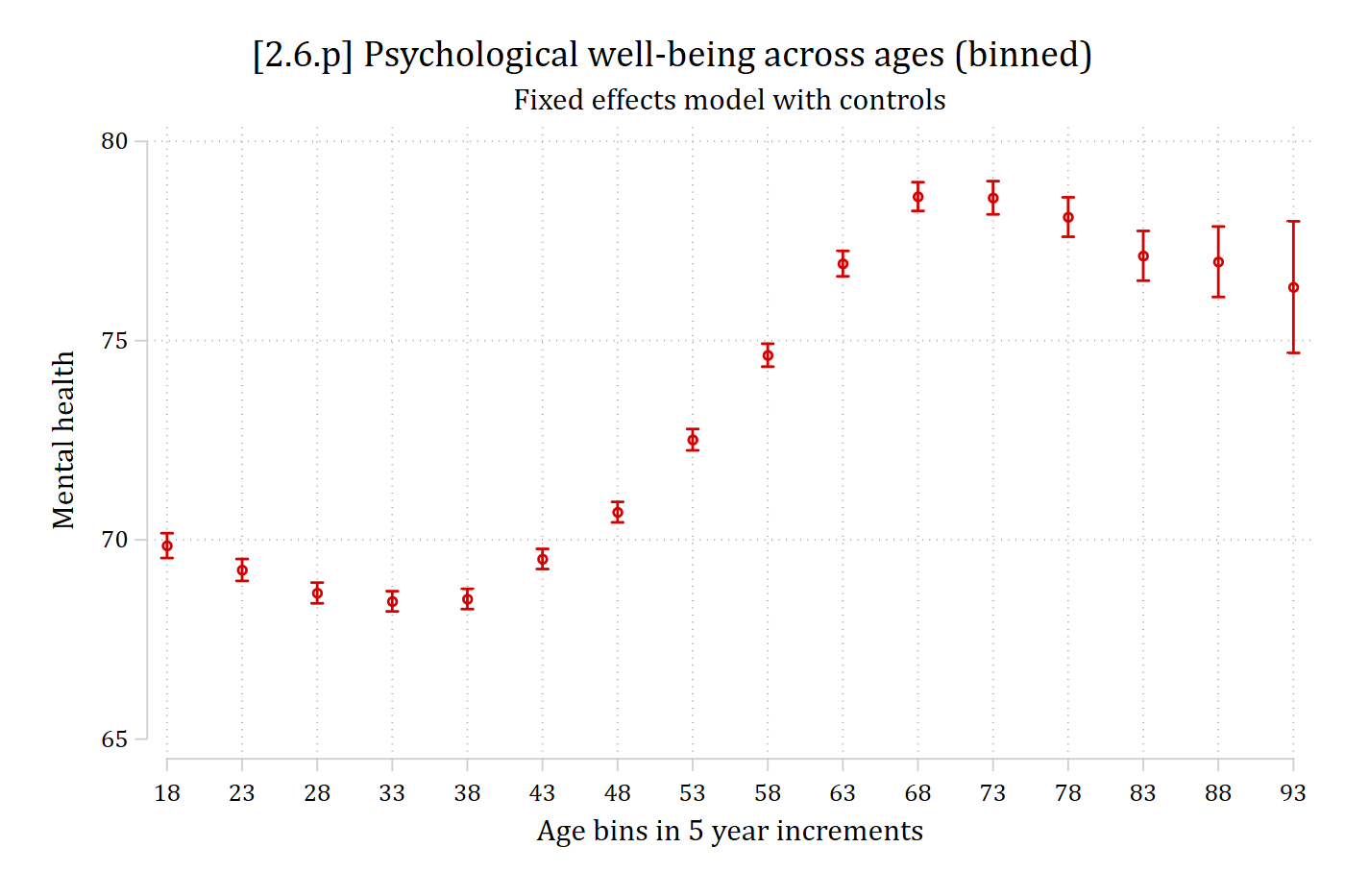
*Note: Two clear “turns” in the slope so need to add both age2 and age3 to model
xtreg MHscale c.age##c.age##c.age ///
    c.oroles##c.oroles c.vroles##c.vroles ///
    c.orolesM c.oroles2M c.vrolesM c.vroles2M ///
    physfunc ib3.educ c.hhincome i.wave, re
Random-effects GLS regression Number of obs = 242,933
Group variable: ID Number of groups = 29,186
R-squared: Obs per group:
Within = 0.0963 min = 1
Between = 0.2652 avg = 8.3
Overall = 0.2412 max = 21
Wald chi2(37) = 33523.87
corr(u_i, X) = 0 (assumed) Prob > chi2 = 0.0000
------------------------------------------------------------------------------
MHscale | Coefficient Std. err. z P>|z| [95% conf. interval]
-------------+----------------------------------------------------------------
age | -1.583 0.046 -34.551 0.000 -1.673 -1.493
|
c.age#c.age | 0.035 0.001 36.961 0.000 0.033 0.037
|
c.age#c.age#|
c.age | -0.000 0.000 -34.643 0.000 -0.000 -0.000
|
oroles | 1.551 0.180 8.637 0.000 1.199 1.902
|
c.oroles#|
c.oroles | -0.118 0.032 -3.684 0.000 -0.181 -0.055
|
vroles | 2.018 0.097 20.844 0.000 1.828 2.208
|
c.vroles#|
c.vroles | -0.290 0.028 -10.257 0.000 -0.345 -0.234
|
orolesM | -0.545 0.477 -1.142 0.253 -1.481 0.391
oroles2M | 0.595 0.092 6.491 0.000 0.415 0.774
vrolesM | 6.598 0.411 16.044 0.000 5.792 7.404
vroles2M | -1.303 0.124 -10.485 0.000 -1.547 -1.059
physfunc | 0.252 0.002 146.057 0.000 0.249 0.256
|
educ |
No HS | -0.903 0.165 -5.466 0.000 -1.227 -0.579
HS | -0.298 0.166 -1.800 0.072 -0.623 0.027
College | 0.835 0.181 4.607 0.000 0.480 1.191
Graduate | 0.791 0.213 3.711 0.000 0.373 1.208
|
hhincome | 0.057 0.006 10.208 0.000 0.046 0.067
|
wave |
3 | -0.329 0.171 -1.927 0.054 -0.664 0.006
4 | -0.618 0.173 -3.571 0.000 -0.957 -0.279
5 | -0.618 0.172 -3.598 0.000 -0.954 -0.281
6 | -0.575 0.175 -3.280 0.001 -0.918 -0.231
7 | -0.740 0.177 -4.185 0.000 -1.087 -0.394
8 | -1.227 0.179 -6.851 0.000 -1.578 -0.876
9 | -0.862 0.178 -4.830 0.000 -1.212 -0.512
10 | -1.539 0.176 -8.734 0.000 -1.884 -1.194
11 | -1.388 0.169 -8.233 0.000 -1.718 -1.058
12 | -1.343 0.170 -7.914 0.000 -1.675 -1.010
13 | -1.505 0.171 -8.814 0.000 -1.840 -1.171
14 | -2.264 0.172 -13.171 0.000 -2.601 -1.927
15 | -2.872 0.174 -16.531 0.000 -3.212 -2.531
16 | -2.783 0.173 -16.077 0.000 -3.122 -2.444
17 | -3.226 0.175 -18.400 0.000 -3.570 -2.882
18 | -3.538 0.178 -19.889 0.000 -3.887 -3.190
19 | -4.260 0.179 -23.797 0.000 -4.611 -3.909
20 | -5.998 0.181 -33.141 0.000 -6.352 -5.643
21 | -6.510 0.184 -35.463 0.000 -6.870 -6.150
22 | -6.267 0.188 -33.418 0.000 -6.635 -5.900
|
_cons | 56.311 0.946 59.538 0.000 54.457 58.164
-------------+----------------------------------------------------------------
sigma_u | 12.617371
sigma_e | 11.655081
rho | .53958312 (fraction of variance due to u_i)
------------------------------------------------------------------------------est store age3_mod
margins, at(age=(18(2)90))Predictive margins Number of obs = 242,933
Model VCE: Conventional
Expression: Linear prediction, predict()
1._at: age = 18
2._at: age = 20
3._at: age = 22
4._at: age = 24
5._at: age = 26
6._at: age = 28
7._at: age = 30
8._at: age = 32
9._at: age = 34
10._at: age = 36
11._at: age = 38
12._at: age = 40
13._at: age = 42
14._at: age = 44
15._at: age = 46
16._at: age = 48
17._at: age = 50
18._at: age = 52
19._at: age = 54
20._at: age = 56
21._at: age = 58
22._at: age = 60
23._at: age = 62
24._at: age = 64
25._at: age = 66
26._at: age = 68
27._at: age = 70
28._at: age = 72
29._at: age = 74
30._at: age = 76
31._at: age = 78
32._at: age = 80
33._at: age = 82
34._at: age = 84
35._at: age = 86
36._at: age = 88
37._at: age = 90
------------------------------------------------------------------------------
| Delta-method
| Margin std. err. z P>|z| [95% conf. interval]
-------------+----------------------------------------------------------------
_at |
1 | 71.206 0.177 402.490 0.000 70.859 71.553
2 | 70.229 0.153 458.707 0.000 69.929 70.529
3 | 69.431 0.135 513.102 0.000 69.166 69.696
4 | 68.801 0.123 559.501 0.000 68.560 69.042
5 | 68.329 0.115 593.493 0.000 68.104 68.555
6 | 68.006 0.111 614.689 0.000 67.789 68.223
7 | 67.821 0.108 626.258 0.000 67.609 68.034
8 | 67.765 0.107 632.622 0.000 67.555 67.975
9 | 67.828 0.106 637.540 0.000 67.619 68.036
10 | 67.999 0.106 643.408 0.000 67.791 68.206
11 | 68.268 0.105 651.321 0.000 68.063 68.474
12 | 68.627 0.104 661.334 0.000 68.423 68.830
13 | 69.064 0.103 672.689 0.000 68.863 69.265
14 | 69.570 0.102 683.986 0.000 69.371 69.770
15 | 70.135 0.101 693.382 0.000 69.937 70.333
16 | 70.749 0.101 698.910 0.000 70.551 70.948
17 | 71.402 0.102 698.913 0.000 71.202 71.602
18 | 72.084 0.104 692.483 0.000 71.880 72.288
19 | 72.785 0.107 679.701 0.000 72.575 72.995
20 | 73.496 0.111 661.546 0.000 73.278 73.713
21 | 74.205 0.116 639.527 0.000 73.978 74.432
22 | 74.904 0.122 615.239 0.000 74.665 75.142
23 | 75.582 0.128 590.018 0.000 75.331 75.833
24 | 76.229 0.135 564.775 0.000 75.965 76.494
25 | 76.836 0.142 539.970 0.000 76.557 77.115
26 | 77.392 0.150 515.669 0.000 77.098 77.686
27 | 77.888 0.158 491.641 0.000 77.577 78.198
28 | 78.313 0.168 467.456 0.000 77.985 78.642
29 | 78.658 0.178 442.606 0.000 78.310 79.007
30 | 78.913 0.189 416.631 0.000 78.542 79.284
31 | 79.067 0.203 389.247 0.000 78.669 79.465
32 | 79.111 0.219 360.451 0.000 78.681 79.541
33 | 79.035 0.239 330.565 0.000 78.567 79.504
34 | 78.829 0.263 300.191 0.000 78.314 79.344
35 | 78.483 0.291 270.084 0.000 77.913 79.052
36 | 77.986 0.324 241.003 0.000 77.352 78.620
37 | 77.330 0.362 213.574 0.000 76.620 78.040
------------------------------------------------------------------------------marginsplot, recastci(rline) ciopt(col(eltblue*.6) lpat(dash)) ///
plotop(msym(none) lcol(eltblue)) xlab(20(10)90) ///
title("[2.6.q] Psychological well-being across ages (cubic specification)"
, size(medlarge)) ///
subtitle("Fixed effects model with controls") ///
xtitle("Age at current wave") ytitle("Mental health")Variables that uniquely identify margins: age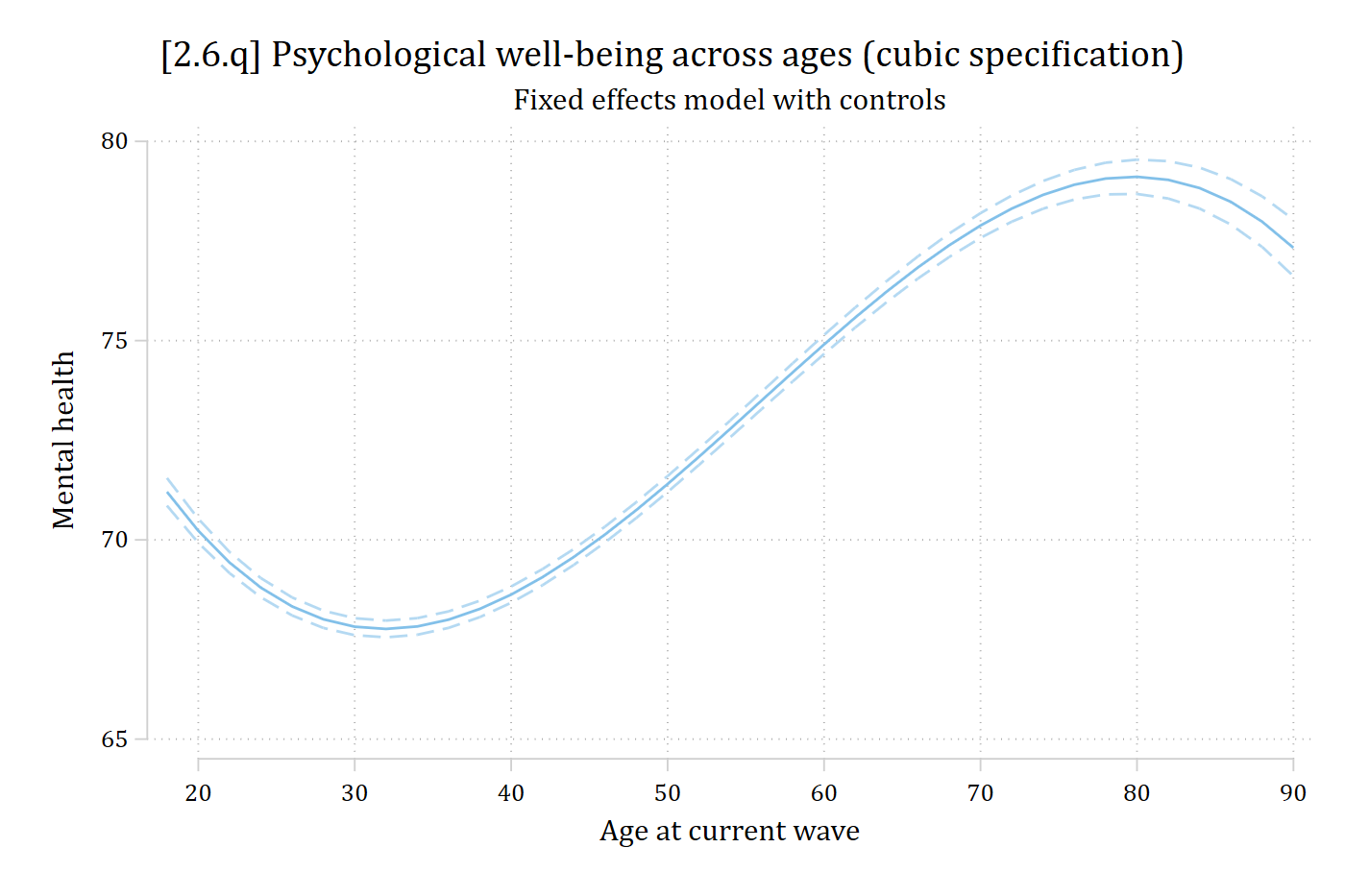
levelsof ageC18 23 28 33 38 43 48 53 58 63 68 73 78 83 88 93global agecats = "`r(levels)'"
preserve
rename age ageold
rename ageC age
qui xtreg MHscale i.age ///
c.oroles##c.oroles c.vroles##c.vroles ///
c.orolesM c.oroles2M c.vrolesM c.vroles2M ///
physfunc ib3.educ c.hhincome i.wave, re
qui margins, at(age=($agecats)) saving(ageC_prs, replace)
restore
est restore age3_mod(results age3_mod are active now)qui margins, at(age=($agecats)) saving(age3_prs, replace)
combomarginsplot ageC_prs age3_prs, ///
labels("Categorical Model" "Cubic Model") ///
title("[2.6.r] Comparison of Predictions for Various Functional Forms of A
ge", size(medium)) ///
ytitle("Mental Health Scale") legend(pos(6) row(1)) Variables that uniquely identify margins: age _filenumber