6.1 Explaining Count Distributions

Overview of count models

  1. Poisson distribution: chance alone explains variation
  2. Poisson regression model: add observed heterogeneity
  3. Negative binomial regression: add unobserved continuous heterogeneity
  4. Zero inflated count models: add unobserved discrete heterogeneity

Overview

  • Start with a Poisson process for modeling counts
    • A series of 0/1 decisions with the rate determined by the mean
  • For Poisson model, let the rate also be determined by observed characteristics
  • This is rarely sufficient so allow unobserved heterogeneity
    • Conceptually, add an error term to the model

A Poisson process

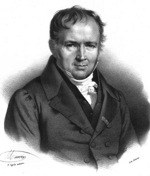
  • Named for Simeon-Denis Poisson
  • The Poisson distribution is a stochastic process
    • Stochastic = randomly determined or “having a random probability distribution or pattern that may be analyzed statistically but may not be predicted precisely”
  • Theoretically, the distribution is the product of a series of yes/no binary choices
    • The shape of the distribution is determined solely by the overall rate (sample mean)

Portrait of Simeon-Denis Poisson.

A figure scratching its head between a green YES button and a red NO button.

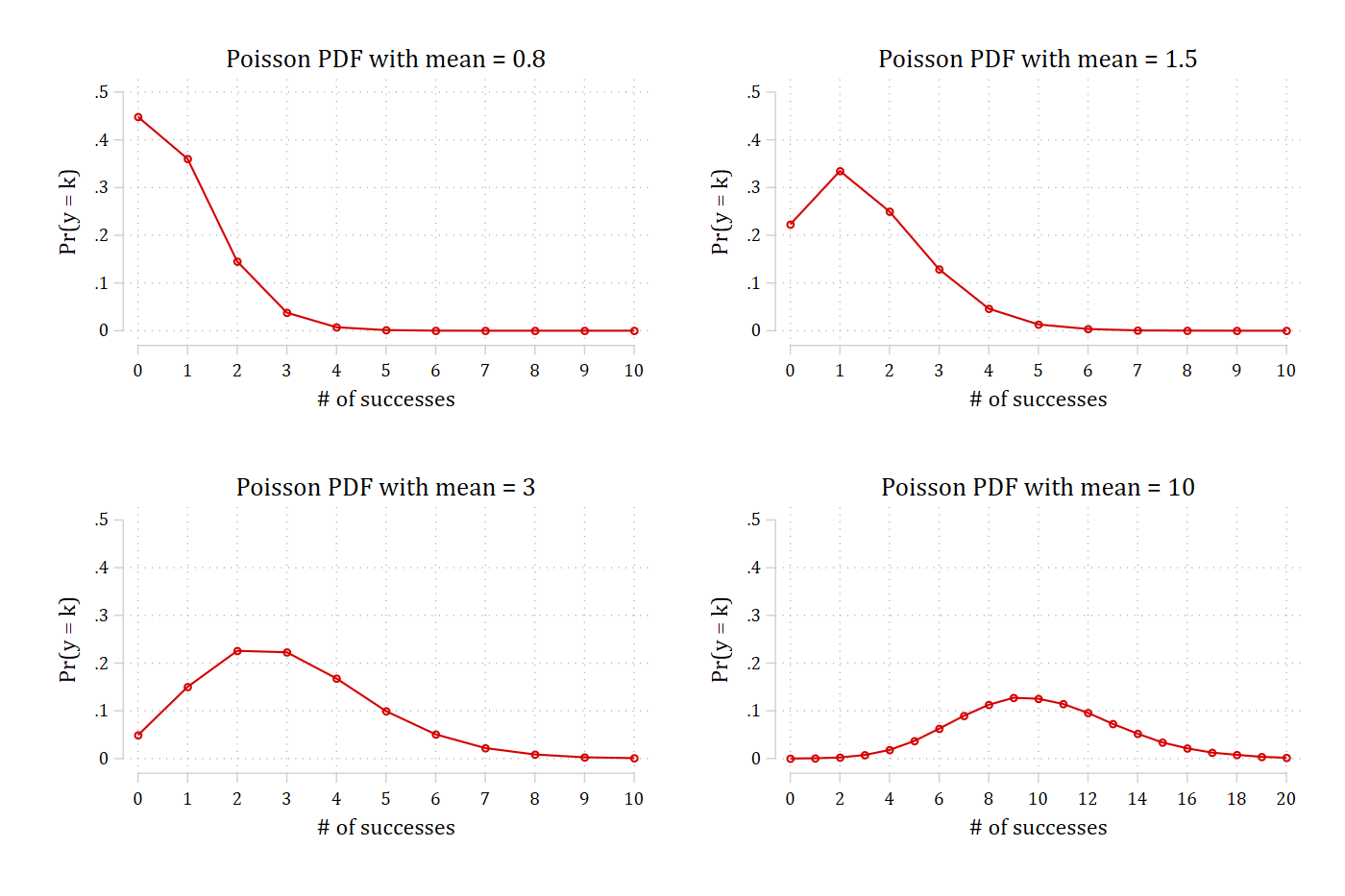
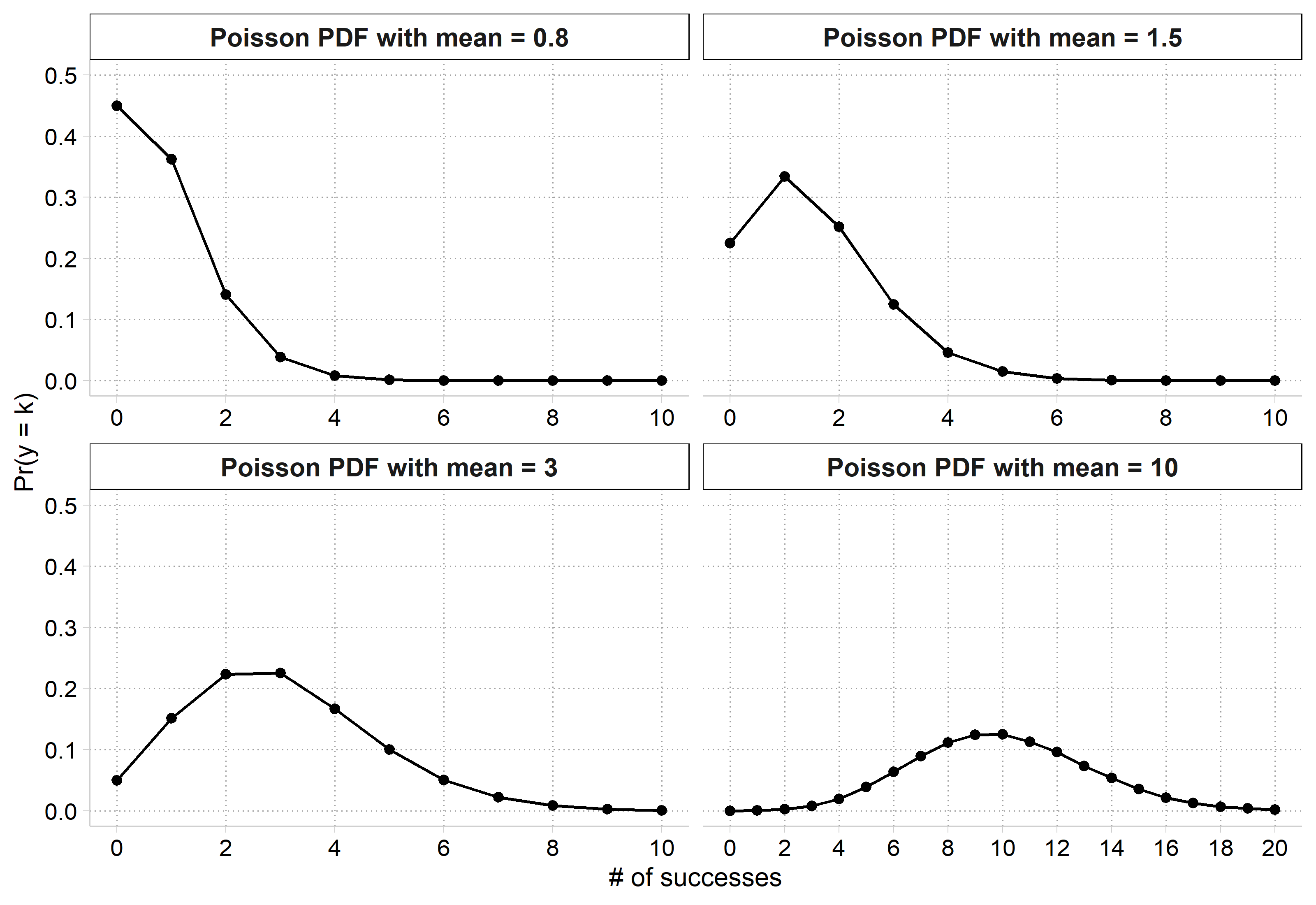
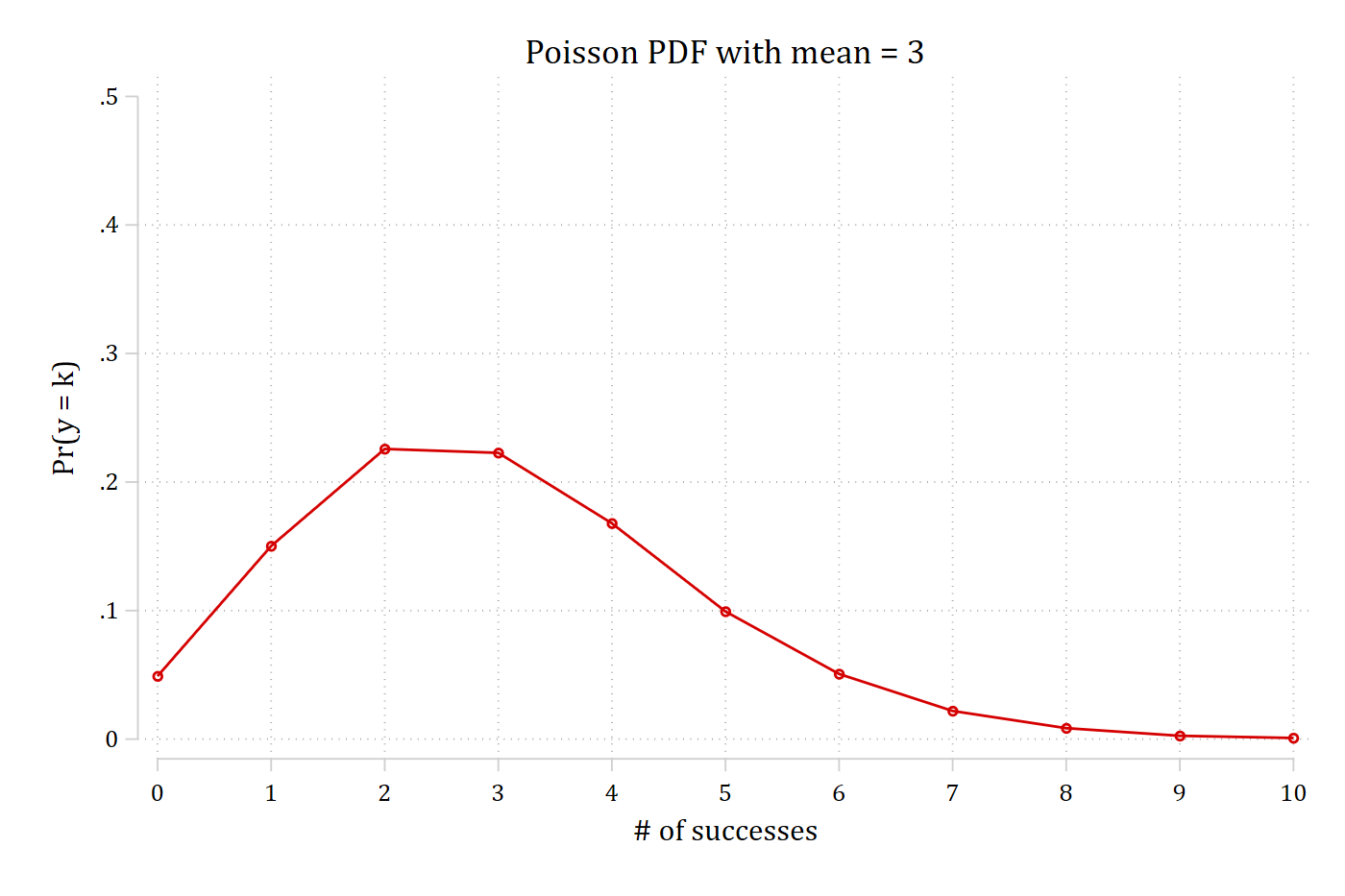
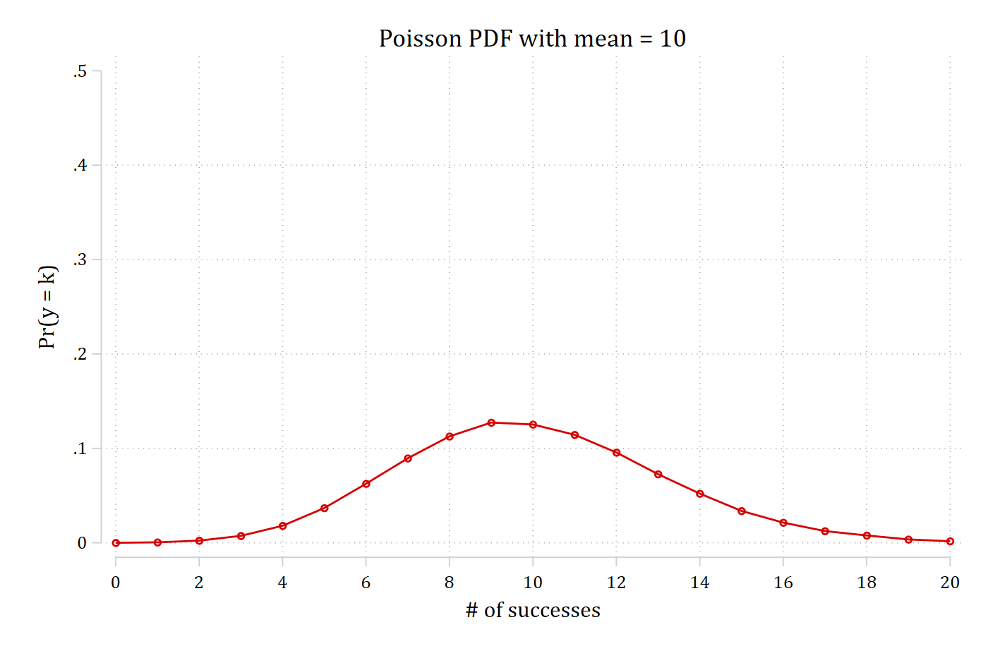
Examples of Poisson PDFs with different means (rates)

*Simulate data to show different Poisson PDFs
clear
set seed 30004
set obs 50000
Number of observations (_N) was 0, now 50,000.
genpoisson y0_8, mu(0.8) adoonly
genpoisson y1_5, mu(1.5) adoonly
genpoisson y3, mu(3) adoonly
genpoisson y4_5, mu(4.5) adoonly
genpoisson y10, mu(10) adoonly
qui poisson y0_8, nolog
qui mgen, pr(0/10) meanpred stub(p08) replace
qui poisson y1_5, nolog
qui mgen, pr(0/10) meanpred stub(p15) replace
qui poisson y3, nolog
qui mgen, pr(0/10) meanpred stub(p3) replace
qui poisson y4_5, nolog
qui mgen, pr(0/10) meanpred stub(p45) replace
qui poisson y10, nolog
qui mgen, pr(0/20) meanpred stub(p10) replace
twoway connected p08obeq p08val, ylab(0(.1).5) xlab(0(1)10) ///
    ytitle("Pr(y = k)") xtitle("# of successes") ///
    title("Poisson PDF with mean = 0.8") saving(mu0_8.gph, replace)
file mu0_8.gph saved
twoway connected p15obeq p15val, ylab(0(.1).5) xlab(0(1)10) ///
    ytitle("Pr(y = k)") xtitle("# of successes") ///
    title("Poisson PDF with mean = 1.5") saving(mu1_5.gph, replace)
file mu1_5.gph saved
twoway connected p3obeq p3val, ylab(0(.1).5) xlab(0(1)10) ///
    ytitle("Pr(y = k)") xtitle("# of successes") ///
    title("Poisson PDF with mean = 3") saving(mu3.gph, replace)
file mu3.gph saved
twoway connected p10obeq p10val, ylab(0(.1).5) xlab(0(2)20) ///
    ytitle("Pr(y = k)") xtitle("# of successes") ///
    title("Poisson PDF with mean = 10") saving(mu10.gph, replace)
file mu10.gph saved
graph combine mu0_8.gph mu1_5.gph mu3.gph mu10.gph

Four panels of Poisson probability distributions from simulated data with means 0.8, 1.5, 3, and 10: with a mean of 0.8 the probability is highest at 0 (about 0.45) and falls quickly; as the mean grows the peak moves right and the distribution spreads out and becomes more symmetric.

library(dplyr)           # data manipulation
library(ggplot2)         # graphs
library(cleanplots)      # graph scheme
cleanplots_defaults()

# Simulate data to show different Poisson PDFs
set.seed(30004)
n <- 50000
sim <- data.frame(y0_8 = rpois(n, 0.8), y1_5 = rpois(n, 1.5), y3 = rpois(n, 3),
  y4_5 = rpois(n, 4.5), y10 = rpois(n, 10))

# Observed proportion of each count, from 0 to maxk
pr_count <- function(y, maxk) data.frame(k = 0:maxk, pr = sapply(0:maxk, function(j) mean(y == j)))

pdfs <- bind_rows(
  "Poisson PDF with mean = 0.8" = pr_count(sim$y0_8, 10),
  "Poisson PDF with mean = 1.5" = pr_count(sim$y1_5, 10),
  "Poisson PDF with mean = 3" = pr_count(sim$y3, 10),
  "Poisson PDF with mean = 10" = pr_count(sim$y10, 20),
  .id = "mean") |>
  mutate(mean = factor(mean, levels = unique(mean)))

ggplot(pdfs, aes(x = k, y = pr)) +
  geom_line() + geom_point() +
  facet_wrap(~ mean, scales = "free_x") +
  scale_x_continuous(breaks = seq(0, 20, 2)) +
  scale_y_continuous(breaks = seq(0, .5, .1), limits = c(0, .5)) +
  labs(x = "# of successes", y = "Pr(y = k)")

Four panels of Poisson probability distributions from simulated data with means 0.8, 1.5, 3, and 10: with a mean of 0.8 the probability is highest at 0 (about 0.45) and falls quickly; as the mean grows the peak moves right and the distribution spreads out and becomes more symmetric.

Formula for Poisson probability density function (PDF)

  • y is a random variable that counts the # of successes
  • Recall some math that is useful here:
    • e = 2.71828...
    • y! = y*(y-1)*(y-2)*...*3*2*1
  • A Poisson distribution defined in terms of the probability of a given value j of the variable y, with the rate μ > 0 is

\[\Pr(y = j\,|\,\mu) = \frac{e^{-\mu}\mu^{j}}{j!}\]

Two cats sitting in a cardboard box that has a drawing of two cat faces and a box added together on its side.

The effect of μ on the Poisson distribution

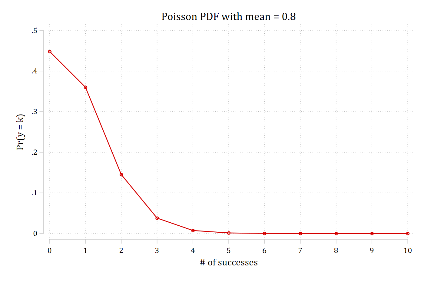
Poisson distribution with mean 0.8: highest probability at 0, falling quickly.

μ = 0.8

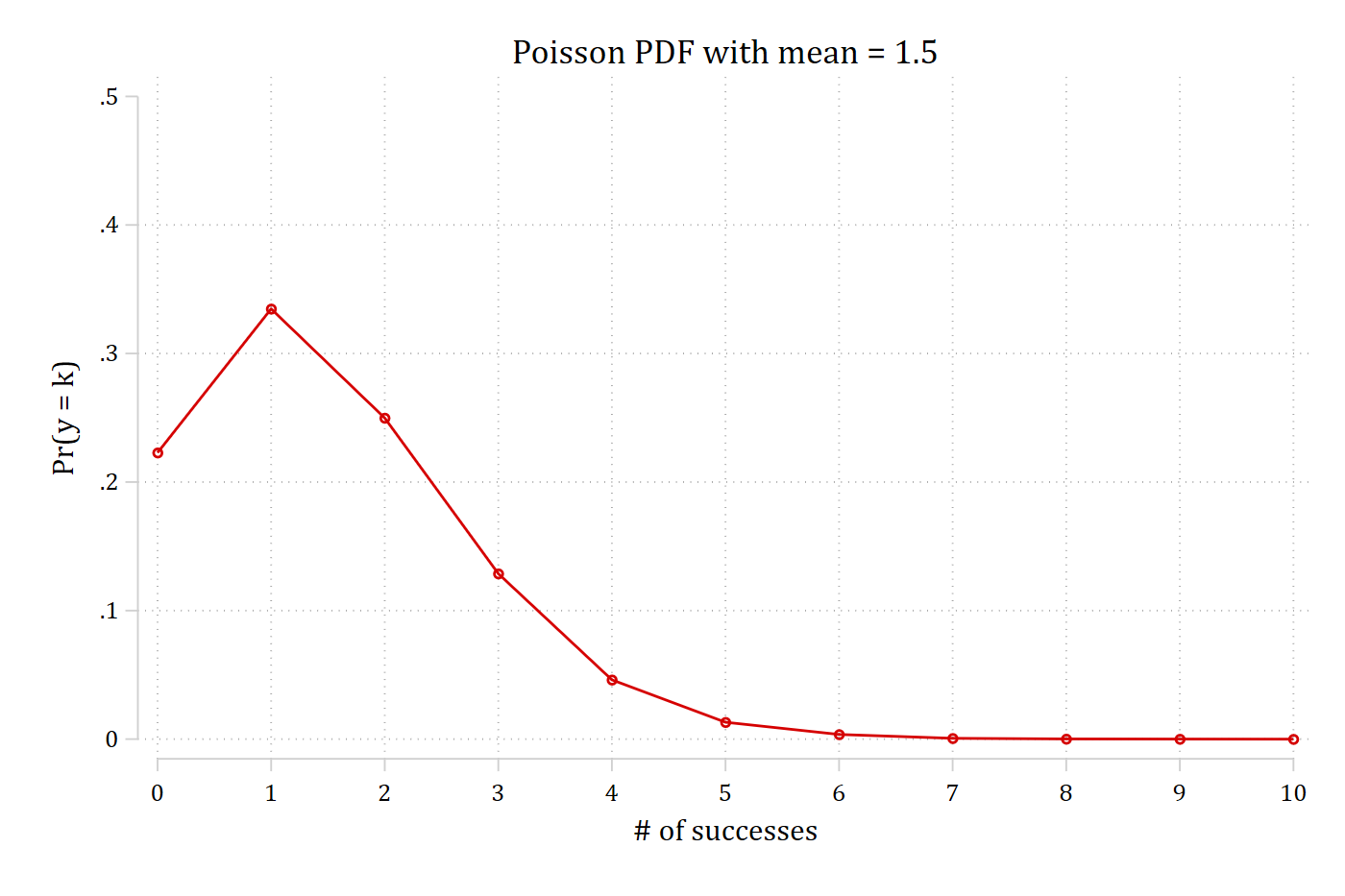
Poisson distribution with mean 1.5: peak at 1.

μ = 1.5

Poisson distribution with mean 3: peak at 2 to 3.

μ = 3

Poisson distribution with mean 10: nearly symmetric around 10.

μ = 10
  • μ is the mean of the count variable, which we call the rate: μ = E(y)
  • As μ increases, mass of distribution moves right
  • With Poisson, the variance is exactly equal to the rate: E(y) = Var(y) = μ
    • Do you expect this to often be reasonable?
  • As μ increases, the distribution becomes mostly symmetrical
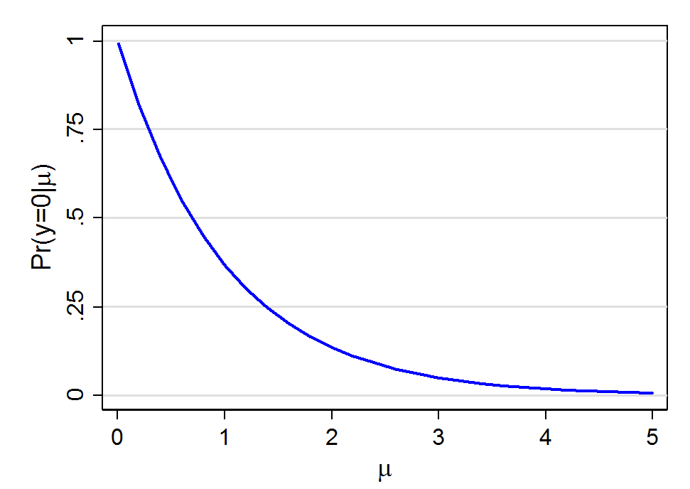
  • As μ increases, the probability of 0’s decreases rapidly as shown below

Poisson distribution and the effect of μ on Pr(y = 0)

Curve of the probability of a zero count against the Poisson mean from 0 to 5: it starts at 1 and falls steeply, to about 0.37 at a mean of 1 and near 0 by a mean of 4.

Poisson distribution implies the number of zeroes in the data declines rapidly for higher mean rates

\[\Pr(y = 0\,|\,\mu = .8) = .45 \qquad \Pr(y = 0\,|\,\mu = 1.5) = .22\]

\[\Pr(y = 0\,|\,\mu = 2.9) = .05 \qquad \Pr(y = 0\,|\,\mu = 10.5) = .00003\]

Why not use linear regression for count outcomes?

  • Counts are sometimes treated as continuous in linear regression
    • Results can be similar with large mean counts
    • Results will diverge most from count model with low mean counts
  • But linear regression is inefficient, inconsistent, and (potentially) biased due to nonlinearity and heteroscedasticity
    • Standard errors will be incorrect
    • Predictions not bounded at zero (i.e., can get negative predictions which are nonsensical)
    • Spurious interactions effects due to assumption of linearity / not respecting floor at zero (Rohrer and Arslan 2021)
    • Linear regression also does not allow for an examination of Pr(y = k) as count models do
  • Count models are almost always preferred
    • Easy to compute
    • (Relatively) easy to interpret
      • More options for interpretation than a linear model
    • Better standard error estimates / more accurate significance tests
    • Ability to account for excess zeros
Back to top