9. Show what the model predicts

Plots of Model Predictions

  • Perhaps the most versatile and useful tool of the applied data analyst is the ability to plot model predictions
    • The most effective way to understand a model is almost always to examine what the model predicts!
      • Predictions are especially important when the model is nonlinear
        • E.g., Because of a quadratic/polynomial term for an IV, because the DV is categorical, etc.
use "https://tdmize.github.io/data/data/gss.dta", clear
(gss.dta | GSS 1972 - 2016 Data | DMV Workshop)
drop if year < 2000
(38,116 observations deleted)
drop if employed != 1
(9,556 observations deleted)
// Linear regression model with age and age-squared
qui regress wages c.age##c.age i.woman i.college i.race
qui margins, at(age=(18(2)90))
// 9.a - Plot predictions for age
marginsplot, plotopts(msym(none)) xlab(20(10)90) ylab(0(5)30) ///
    recastci(rline) ciopts(lpat(dash) col(gs12)) ///
    ytitle("Hourly Wages") xtitle("Age in Years") ///
    title("[9.a] Predicted Hourly Wages Based on Age of Worker")
Variables that uniquely identify margins: age

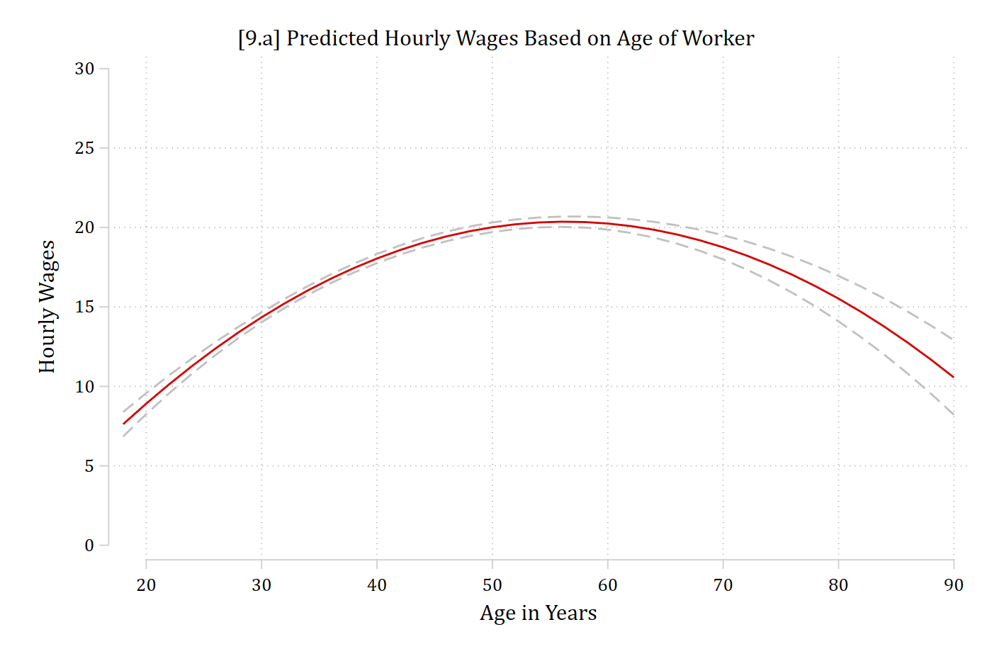
[9.a] Predicted hourly wages by age from 18 to 90 with a dashed 95% confidence interval: wages rise from about 8 dollars at 18 to a peak of about 20 dollars in the mid-50s and then fall to about 11 dollars at 90.

library(foreign)            # load Stata datasets
library(ggplot2)            # main graphics package
library(dplyr)              # data manipulation tools
library(marginaleffects)    # predictions and marginal effects
library(cleanplots)         # Mize's graphics scheme

## Use cleanplots colors, markers, lines, and theme for all graphs ##
cleanplots_defaults()
theme_update(plot.title.position = "plot")   # titles start at left edge of graph

# General Social Survey Data
gss <- droplevels(read.dta("https://tdmize.github.io/data/data/gss.dta"))
gss_emp <- droplevels(filter(gss, year >= 2000, employed == 1))

# Linear regression model with age and age-squared
wage_mod <- lm(wages ~ poly(age, 2, raw = TRUE) + woman + college + race, data = gss_emp)

# 9.a - Plot predictions for age
plot_predictions(wage_mod, condition = "age") +
  labs(x = "Age in Years", y = "Hourly Wages",
       title = "[9.a] Predicted Hourly Wages Based on Age of Worker") +
  scale_x_continuous(breaks = seq(20, 90, 10)) +
  scale_y_continuous(breaks = seq(0, 30, 5)) + coord_cartesian(ylim = c(0, 30))

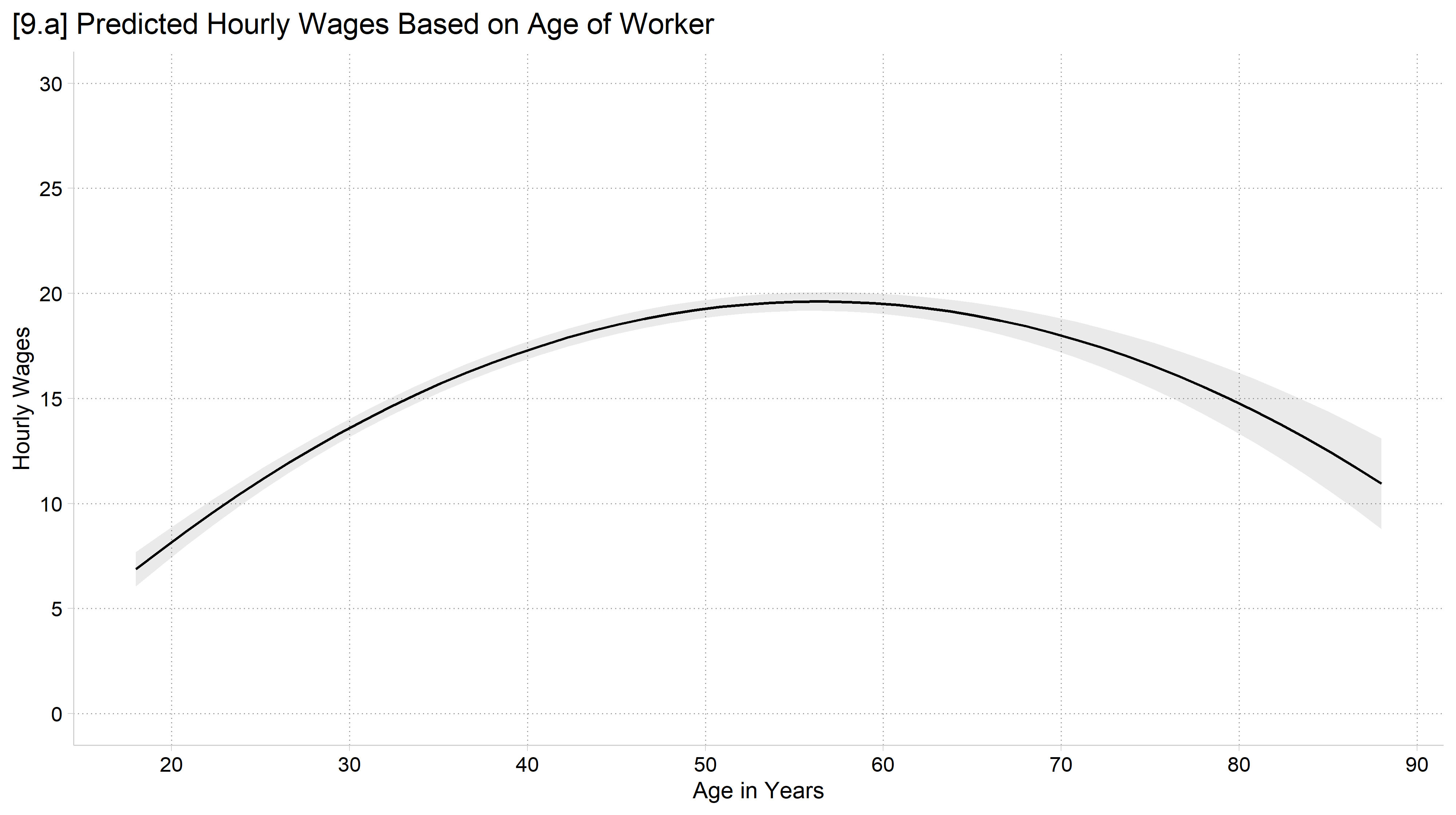
[9.a] Predicted hourly wages by age from 18 to 90 with a 95% confidence interval: wages rise to a peak in the mid-50s and then fall.

Adding distributional information

// Allow the age effect to differ for men and women
qui regress wages c.age##c.age##i.woman i.college i.race
qui margins, at(age=(18(2)90) woman=(0 1))
// 9.b - Histogram to show distribution of age
marginsplot, plotopts(msym(i)) ///
    recastci(rline) ciopts(lpat(dash) col(gs12)) ///
    ytitle("Hourly Wages") xtitle("Age in Years") ///
    title("[9.b] Predicted Hourly Wages Based on Age of Worker") ///
    addplot(hist age, width(1) lcol(gs10) ///
    fcol(none) yaxis(2) yscale(range(0 0.15) off alt axis(2)) ///
    legend(order(3 "Men" 4 "Women")) xlab(20(10)90) ylab(0(5)30))
Variables that uniquely identify margins: age woman

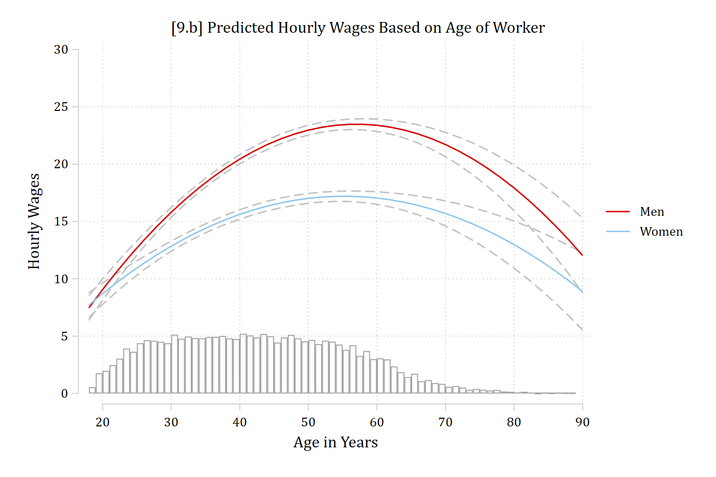
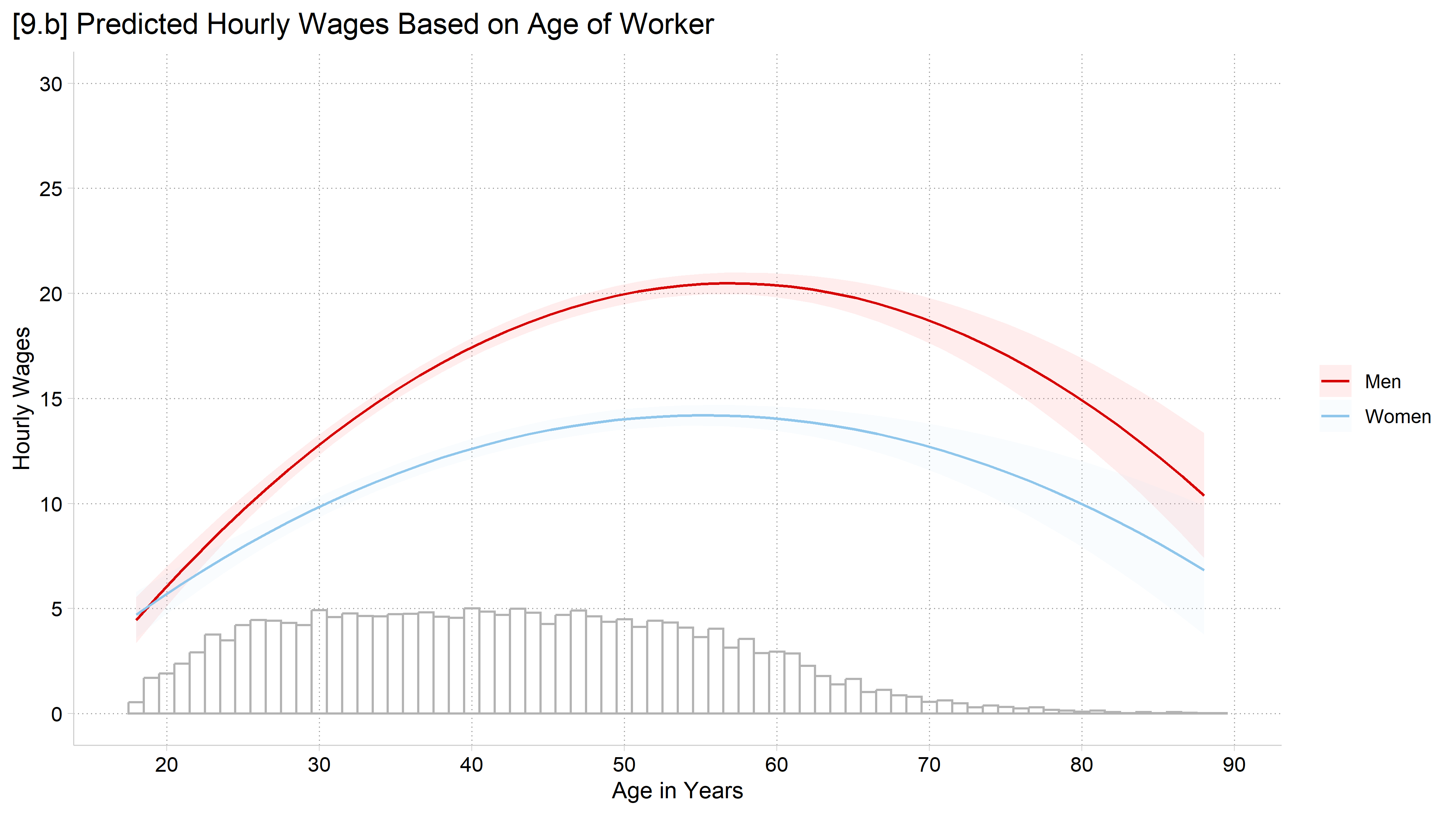
[9.b] Predicted hourly wages by age for men and women with 95% confidence intervals, and a histogram of age along the bottom of the graph: most workers are between about 20 and 65, and few are older than 70, where the confidence intervals widen.

# Allow the age effect to differ for men and women
wage_int <- lm(wages ~ poly(age, 2, raw = TRUE) * woman + college + race, data = gss_emp)

# 9.b - Add a histogram of age to the bottom of the plot
plot_predictions(wage_int, condition = c("age", "woman")) +
  geom_histogram(data = gss_emp, binwidth = 1, fill = NA, color = "gray70",
                 aes(x = age, y = after_stat(count / max(count) * 5)),
                 inherit.aes = FALSE) +
  labs(x = "Age in Years", y = "Hourly Wages", color = "", fill = "",
       title = "[9.b] Predicted Hourly Wages Based on Age of Worker") +
  scale_x_continuous(breaks = seq(20, 90, 10)) +
  scale_y_continuous(breaks = seq(0, 30, 5)) + coord_cartesian(ylim = c(0, 30))

[9.b] Predicted hourly wages by age for men and women with 95% confidence intervals, and a histogram of age along the bottom of the graph: most workers are between about 20 and 65, and few are older than 70, where the confidence intervals widen.

// Generate variables to make rugs on plot
gen pipe = "|" if age != .     // What rug looks like
gen agerand = age + rnormal(0,1) // "jitter" age
(56 missing values generated)
gen where = 0                  // Where on y-axis to put 1st rug
gen where2 = 1.2               // Where on y-axis to put 2nd rug
// 9.c - Rug plots: separate rugs for men and women (faded colors)
marginsplot, plotopts(msym(i)) ///
    recastci(rline) ciopts(lpat(dash) col(gs12)) ///
    ytitle("Hourly Wages") xtitle("Age in Years") ///
    title("[9.c] Predicted Hourly Wages Based on Age of Worker") ///
    addplot(scatter where2 agerand if woman == 0, ///
        ms(none) mlabel(pipe) mlabcol(red*.6) mlabpos(0) || ///
    scatter where agerand if woman == 1, ///
        ms(none) mlabel(pipe) mlabcol(eltblue*.6) mlabpos(0) ///
    legend(order(3 "Men" 4 "Women")) xlab(20(10)90) ylab(0(5)30))
Variables that uniquely identify margins: age woman

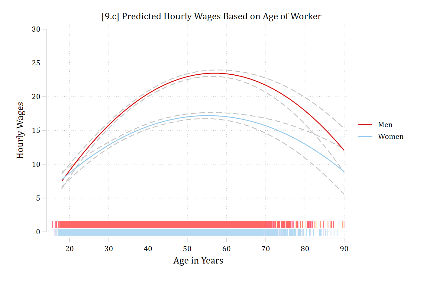
[9.c] The same predictions with two rug plots along the bottom, a faded red rug for men and a faded blue rug for women: each tick marks a worker's (jittered) age, so the rugs are densest between about 20 and 65.

# 9.c - Rug plot: "jitter" age so can better see where the data is; colors faded
dat_rug <- insight::get_data(wage_int)                          # estimation sample
dat_rug$age_j <- dat_rug$age + runif(nrow(dat_rug), -0.4, 0.4)  # jitter
dat_rug$rug_y <- ifelse(dat_rug$woman == "Men", 1.2, 0)         # men's rug above women's

plot_predictions(wage_int, condition = c("age", "woman")) +
  geom_point(data = dat_rug, aes(x = age_j, y = rug_y, color = woman), shape = "|",
             size = 3, alpha = 0.06, inherit.aes = FALSE, show.legend = FALSE) +
  labs(x = "Age in Years", y = "Hourly Wages", color = "", fill = "",
       title = "[9.c] Predicted Hourly Wages Based on Age of Worker",
       subtitle = "With rug plot to show distribution of age (jittered)") +
  scale_x_continuous(breaks = seq(20, 90, 10)) +
  scale_y_continuous(breaks = seq(0, 30, 5)) + coord_cartesian(ylim = c(0, 30))

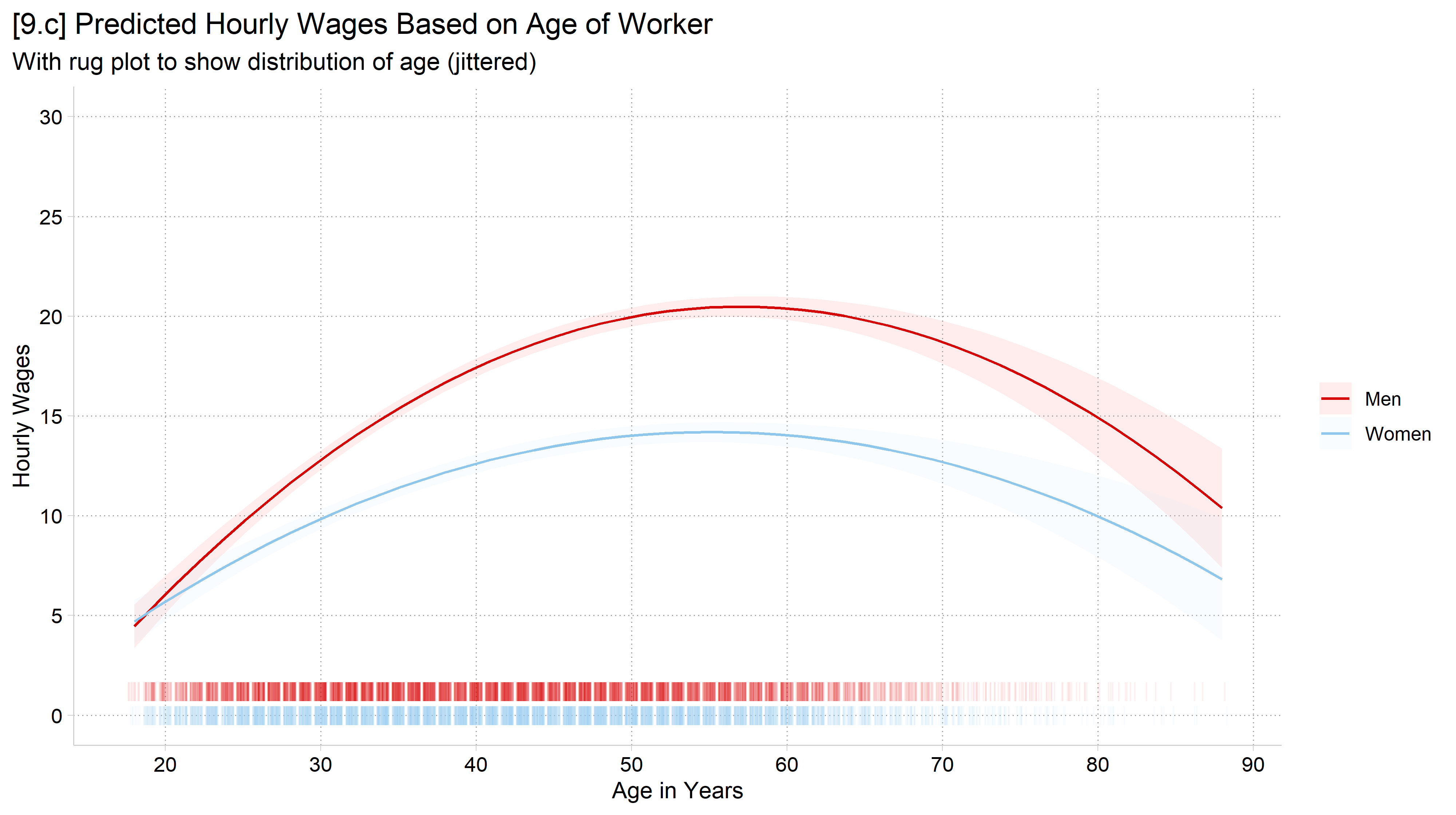
[9.c] The same predictions with two rug plots along the bottom, a faded red rug for men above a faded blue rug for women: each tick marks a worker's (jittered) age, so the rugs are densest between about 20 and 65.

Plotting predictions for nominal vs continuous variables

  • For IVs treated as continuous: sort the x-axis left to right by values of the IV, make predictions at most or all levels of the IV, and connect the lines between the predictions
    • This helps visually mirror the assumption of continuity in how you modeled the IV
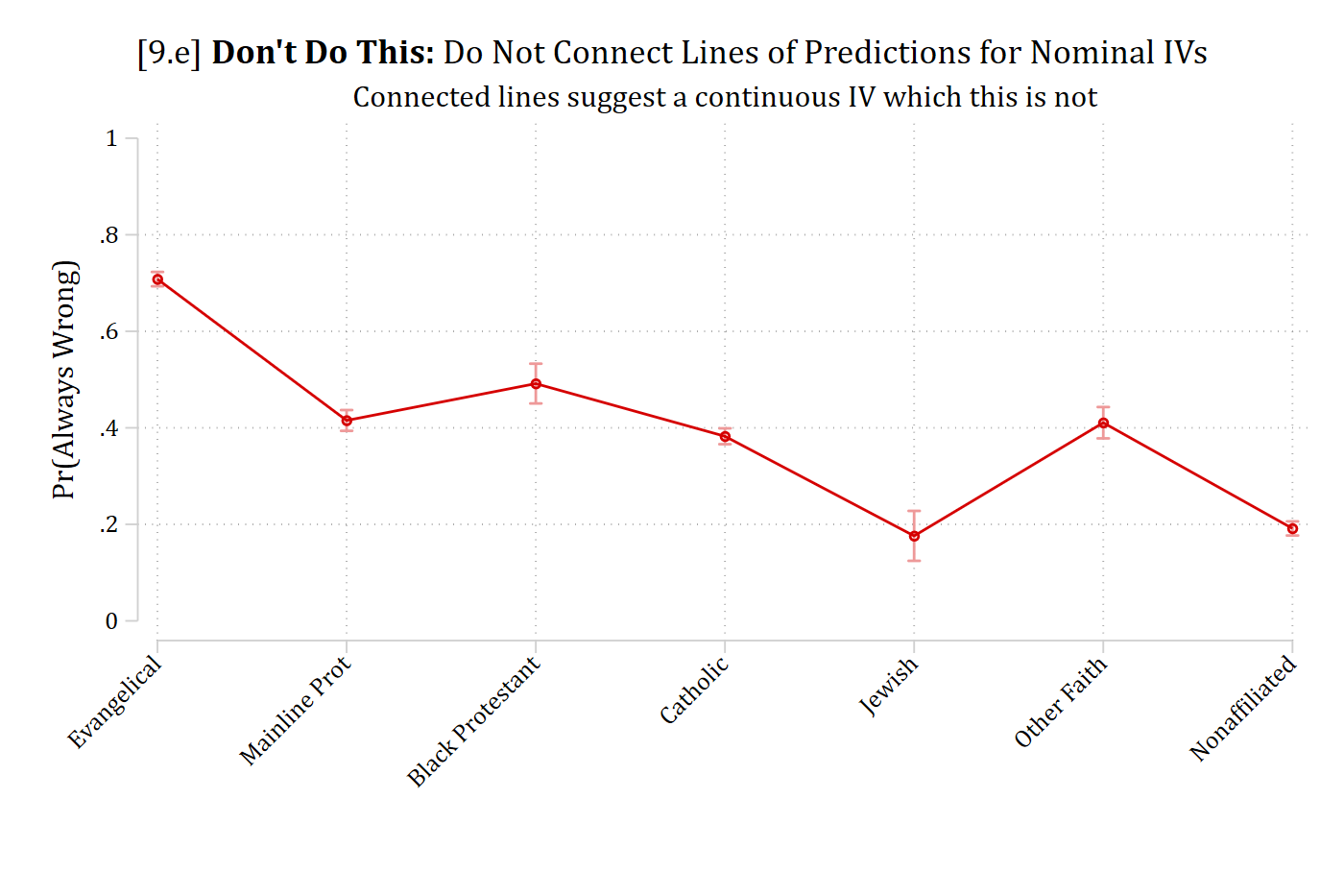
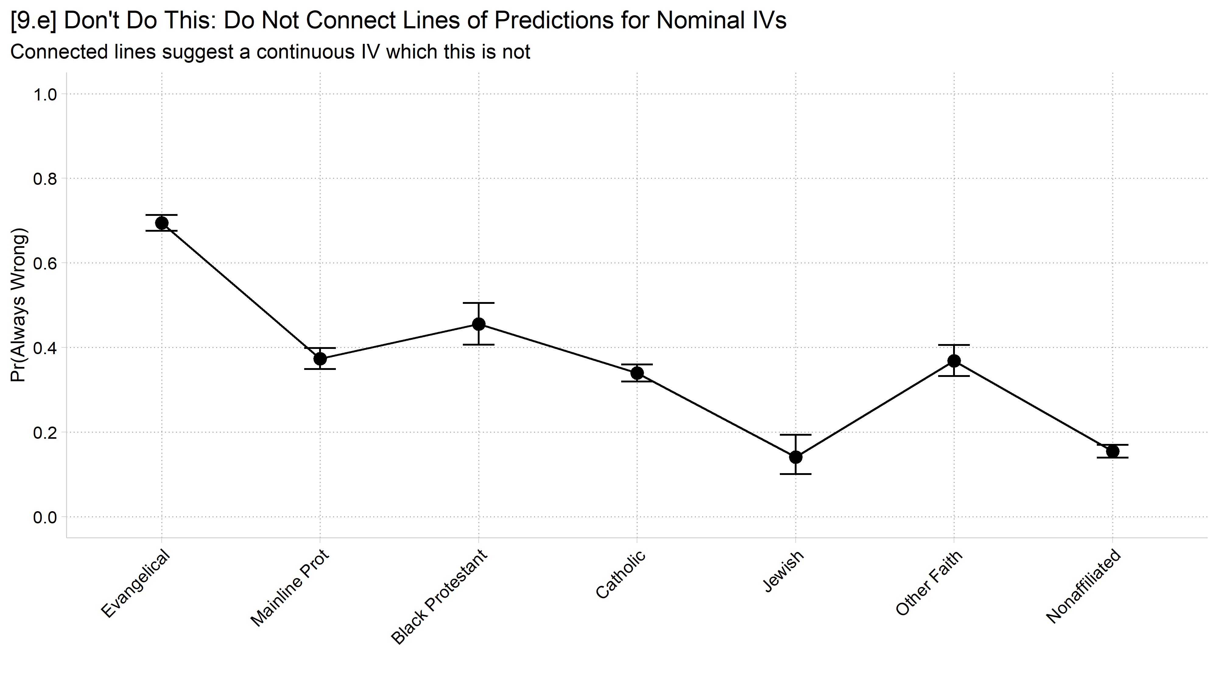
  • For IVs treated as nominal: x-axis sorting is often arbitrary*, dots or bars should clearly represent distinct predictions being made for each grouping, and there should be no lines connecting the predictions
    • Lines connecting predictions suggest continuity, whereas nominal IVs have no ordering information
    • Be consistent in ordering across figures, tables, etc.
  • For ordinal variables modeled as nominal, use the logical order in tables and graphs (e.g., “high school degree” left of “college degree”)
use "https://tdmize.github.io/data/data/cda_gss.dta", clear
(cda_gss.dta |  GSS 1972-2021 CDA - Categorical Data Analysis | date created 202
> 3)
tab samesexop
 Opinion of Same-Sex |
       Relationships |      Freq.     Percent        Cum.
---------------------+-----------------------------------
        always wrong |     24,162       60.00       60.00
 almost always wrong |      1,868        4.64       64.64
wrong only sometimes |      2,739        6.80       71.44
    not wrong at all |     11,501       28.56      100.00
---------------------+-----------------------------------
               Total |     40,270      100.00
gen samesexAW = samesexop
(28,576 missing values generated)
lab var samesexAW "Same Sex Relationship Always Wrong"
recode samesexAW 1=1 2/4 = 0
(16,108 changes made to samesexAW)
lab def ssaw 0"Not Always Wrong" 1"Always Wrong"
lab val samesexAW ssaw
tab samesexop samesexAW
                     | Same Sex Relationship
 Opinion of Same-Sex |     Always Wrong
       Relationships | Not Alway  Always Wr |     Total
---------------------+----------------------+----------
        always wrong |         0     24,162 |    24,162 
 almost always wrong |     1,868          0 |     1,868 
wrong only sometimes |     2,739          0 |     2,739 
    not wrong at all |    11,501          0 |    11,501 
---------------------+----------------------+----------
               Total |    16,108     24,162 |    40,270 
drop if missing(samesexAW, reltrad, woman, college, race3, faminc, age, year)
(34,086 observations deleted)
*Omitting Catholic -- Only including surveys beginning in 2000
qui logit samesexAW ib4.reltrad i.woman i.college i.race3 c.faminc c.age ///
    if year >= 2000
*Get predictions for each category
margins reltrad
Predictive margins                                      Number of obs = 13,830
Model VCE: OIM

Expression: Pr(samesexAW), predict()

-------------------------------------------------------------------------------
              |            Delta-method
              |     Margin   std. err.      z    P>|z|     [95% conf. interval]
--------------+----------------------------------------------------------------
      reltrad |
 Evangelical  |      0.708      0.008   93.334   0.000        0.693       0.723
Mainline P..  |      0.415      0.011   37.742   0.000        0.394       0.437
Black Prot..  |      0.492      0.021   23.404   0.000        0.451       0.533
    Catholic  |      0.383      0.008   45.654   0.000        0.366       0.399
      Jewish  |      0.176      0.026    6.674   0.000        0.124       0.228
 Other Faith  |      0.411      0.017   24.803   0.000        0.378       0.443
Nonaffilia~d  |      0.192      0.007   25.773   0.000        0.177       0.206
-------------------------------------------------------------------------------
// 9.d - Use recast(scatter) for a dot plot for a nominal IV
marginsplot, recast(scatter) ylab(0(.2)1) ciopts(col(*.4)) xtitle(" ") ///
    xlab(, angle(45)) ytitle("Pr(Always Wrong)") ///
    title("[9.d] Predicted Probability of Viewing Same-Sex Relationships As 'A
lways Wrong'", size(medium)) ///
    subtitle("By Religious Affiliation")
Variables that uniquely identify margins: reltrad

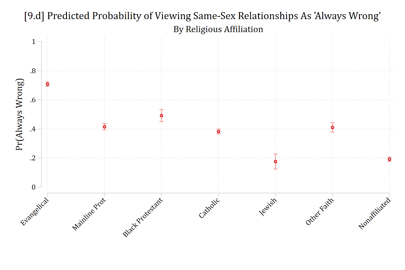
[9.d] Dot plot of the predicted probability of viewing same-sex relationships as always wrong for seven religious traditions, with 95% confidence intervals: highest for Evangelicals (about .71), about .38 to .49 for Mainline Protestants, Black Protestants, Catholics, and Other Faith, and lowest for Jewish (.18) and Nonaffiliated (.19) respondents.

# General Social Survey Data (religious tradition ex)
cda_gss <- droplevels(read.dta("https://tdmize.github.io/data/data/cda_gss.dta"))

# DV: same-sex relationships are always wrong (1) vs not (0)
cda_gss$samesexAW <- as.numeric(cda_gss$samesexop == "always wrong")

gss_rel <- cda_gss %>%
  filter(year >= 2000) %>%
  filter(!is.na(samesexAW), !is.na(reltrad), !is.na(woman), !is.na(college),
         !is.na(race3), !is.na(faminc), !is.na(age)) %>%
  droplevels()

logit_rel <- glm(samesexAW ~ reltrad + woman + college + race3 + faminc + age,
                 family = binomial, data = gss_rel)

# 9.d - The default plot for a nominal IV is a dot plot (which is good)
plot_predictions(logit_rel, condition = "reltrad") +
  labs(x = "", y = "Pr(Always Wrong)",
       title = "[9.d] Predicted Probability of Viewing Same-Sex Relationships As 'Always Wrong'",
       subtitle = "By Religious Affiliation") +
  scale_y_continuous(breaks = seq(0, 1, .2), limits = c(0, 1)) +
  scale_x_discrete(guide = guide_axis(angle = 45))

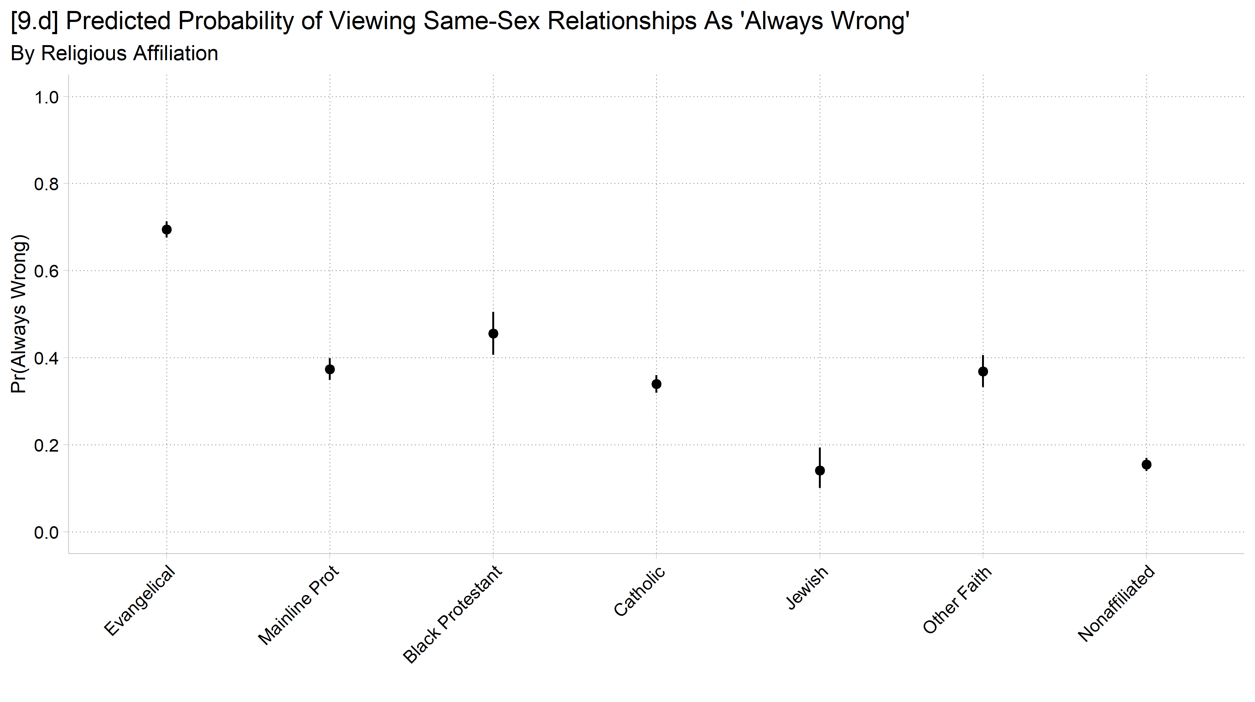
[9.d] Dot plot of the predicted probability of viewing same-sex relationships as always wrong for seven religious traditions, with 95% confidence intervals: highest for Evangelicals and lowest for Jewish and Nonaffiliated respondents.

// 9.e - DON'T DO THIS! marginsplot's default connects lines for a nominal IV
marginsplot, ylab(0(.2)1) ciopts(col(*.4)) xtitle(" ") ///
    xlab(, angle(45)) ytitle("Pr(Always Wrong)") ///
    title("[9.e] {bf:Don't Do This:} Do Not Connect Lines of Predictions for N
ominal IVs", size(medium)) ///
    subtitle("Connected lines suggest a continuous IV which this is not")
Variables that uniquely identify margins: reltrad

[9.e] Don't do this: the same predicted probabilities for the seven religious traditions connected by a line, which wrongly suggests the religious traditions are ordered.

# 9.e - DON'T DO THIS! Connected lines suggest a continuous IV, which this is not
pred_rel <- plot_predictions(logit_rel, condition = "reltrad", draw = FALSE)

ggplot(pred_rel, aes(x = reltrad, y = estimate, group = 1)) +
  geom_line() +
  geom_point(size = 3) +
  geom_errorbar(aes(ymin = conf.low, ymax = conf.high), width = .2) +
  labs(x = "", y = "Pr(Always Wrong)",
       title = "[9.e] Don't Do This: Do Not Connect Lines of Predictions for Nominal IVs",
       subtitle = "Connected lines suggest a continuous IV which this is not") +
  scale_y_continuous(breaks = seq(0, 1, .2), limits = c(0, 1)) +
  scale_x_discrete(guide = guide_axis(angle = 45))

[9.e] Don't do this: the same predicted probabilities for the seven religious traditions connected by a line, which wrongly suggests the religious traditions are ordered.

// 9.f - A bar chart is an equally good alternative
marginsplot, recast(bar) plotopts(barw(.6) color(ltblue)) ylab(0(.2)1) ciopts(
color(gs8)) ///
    xtitle(" ") xlab(, angle(45)) ytitle("Pr(Always Wrong)") ///
    title("[9.f] Predicted Probability of Viewing Same-Sex Relationships As 'A
lways Wrong'", size(medium)) ///
    subtitle("By Religious Affiliation")
Variables that uniquely identify margins: reltrad

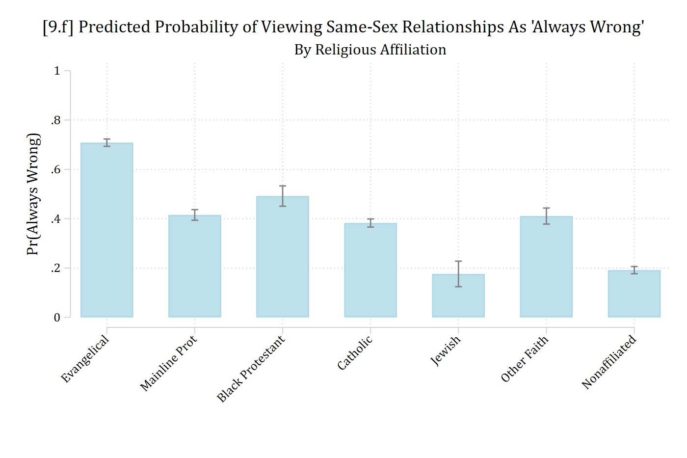
[9.f] The same predicted probabilities for the seven religious traditions as a light blue bar chart with 95% confidence intervals.

# 9.f - A bar chart is an equally good alternative
ggplot(pred_rel, aes(x = reltrad, y = estimate)) +
  geom_col(fill = cleanplots_colors("ltblue", bars = TRUE), width = .6) +
  geom_errorbar(aes(ymin = conf.low, ymax = conf.high), width = .2, color = "gray40") +
  labs(x = "", y = "Pr(Always Wrong)",
       title = "[9.f] Predicted Probability of Viewing Same-Sex Relationships As 'Always Wrong'",
       subtitle = "By Religious Affiliation") +
  scale_y_continuous(breaks = seq(0, 1, .2), limits = c(0, 1)) +
  scale_x_discrete(guide = guide_axis(angle = 45))

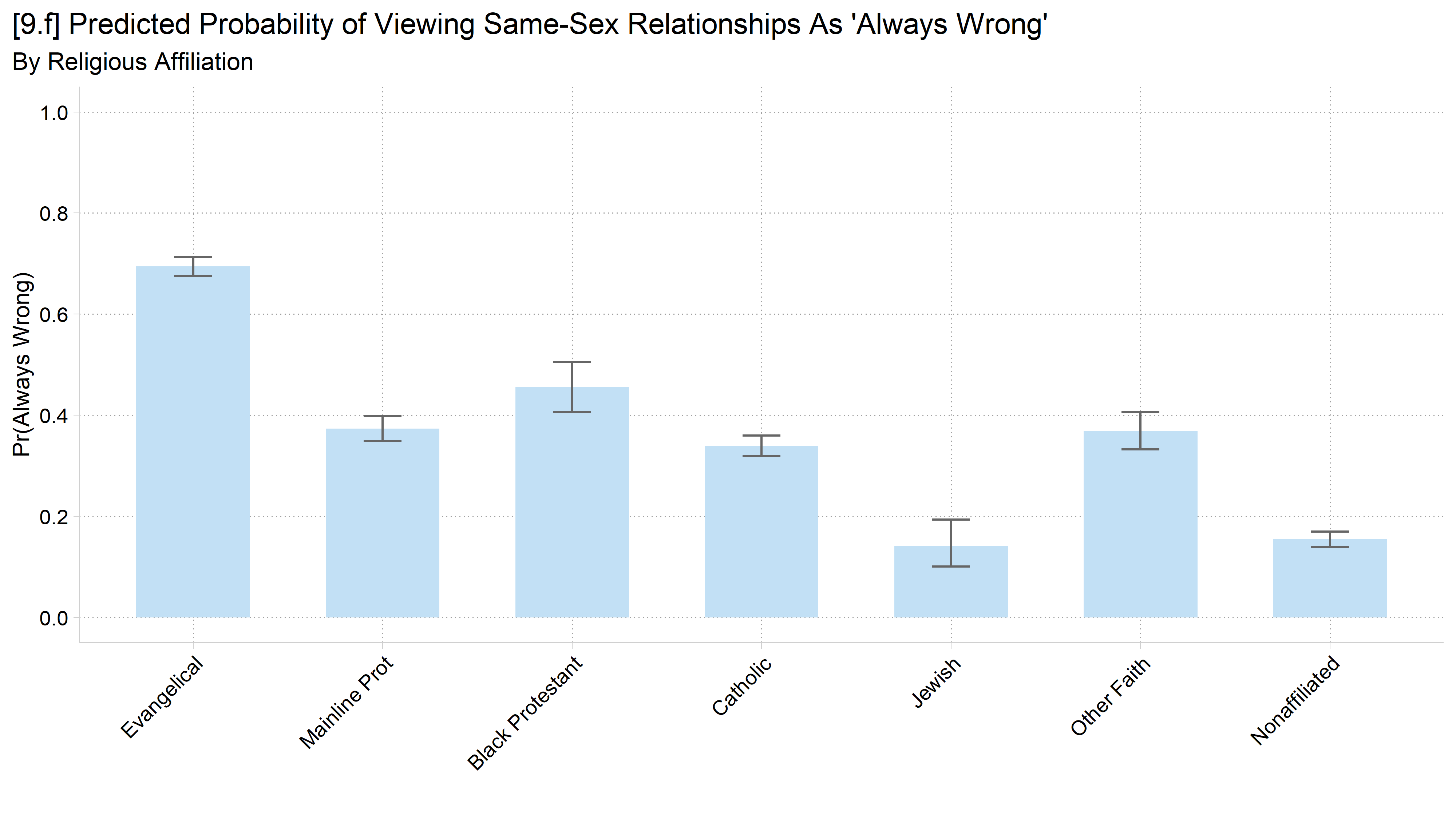
[9.f] The same predicted probabilities for the seven religious traditions as a light blue bar chart with 95% confidence intervals.

Confidence intervals and statistical significance

  • “Fun” game: guess which of the following group differences (b0 vs. b1) are significant at the 95% level (two-tailed test)
  • The dependent variable is continuous
    • The independent variable (b) is binary with two values (0 and 1)
  • The test for significance can be*:
    • A t-test
    • An ANOVA
    • A linear regression model
    • A Wald test for equality of predictions

*Fun fact: these are all identical tests in this simple case…

Meme of several Spider-Men pointing at each other.

// Simulated data: two groups (b = 0 vs b = 1) with a true difference of 5
clear
set seed 30004
set obs 1000
Number of observations (_N) was 0, now 1,000.
gen b = .
(1,000 missing values generated)
replace b = 0 in 1/500
(500 real changes made)
replace b = 1 in 501/1000
(500 real changes made)
gen y10 = 50 + 5*b + rnormal(0,10)
gen y20 = 50 + 5*b + rnormal(0,20)
gen y25 = 50 + 5*b + rnormal(0,25)
gen y30 = 50 + 5*b + rnormal(0,30)
* Estimate the models and save the predictions for each outcome
foreach y in y30 y20 y25 {
    qui reg `y' i.b
    qui margins, at(b=(0 1)) post
    est store pr_`y'
}
// 9.g - Error term has SD of 30
est restore pr_y30
(results pr_y30 are active now)
coefplot, vertical ciop(recast(rcap) col(gs10)) ylab(45(1)60) ///
    xlab(1 "b = 0" 2 "b = 1") ytitle("y-hat") ///
    title("[9.g] Predictions and 95% Confidence Intervals - Linear Regression 
Model")

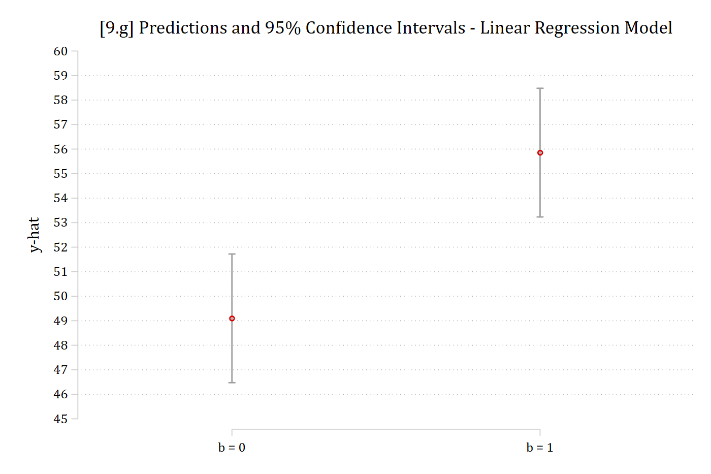
[9.g] Predicted y and 95% confidence intervals for b = 0 (about 49.1) and b = 1 (about 55.9): the two confidence intervals do not overlap.

# Simulated data: two groups (b = 0 vs b = 1) with a true difference of 5
# R and Stata draw different random numbers; this seed gives the same pattern as Stata's
set.seed(43940)
sim <- data.frame(b = factor(rep(c(0, 1), each = 500)))
sim$y10 <- 50 + 5 * (sim$b == 1) + rnorm(1000, 0, 10)
sim$y20 <- 50 + 5 * (sim$b == 1) + rnorm(1000, 0, 20)
sim$y25 <- 50 + 5 * (sim$b == 1) + rnorm(1000, 0, 25)
sim$y30 <- 50 + 5 * (sim$b == 1) + rnorm(1000, 0, 30)

# Plot predictions and CIs for the two groups; optionally show the test of the difference
ci_plot <- function(y, label, show_p = FALSE) {
  m <- lm(reformulate("b", y), data = sim)
  p <- avg_comparisons(m, variables = "b")$p.value
  ggplot(avg_predictions(m, variables = "b"), aes(x = b, y = estimate)) +
    geom_point(size = 3) +
    geom_errorbar(aes(ymin = conf.low, ymax = conf.high), width = .1, color = "gray60") +
    scale_x_discrete(labels = c("b = 0", "b = 1")) +
    scale_y_continuous(breaks = seq(45, 60, 1)) + coord_cartesian(ylim = c(45, 60)) +
    labs(x = "", y = "y-hat",
         title = paste0("[", label, "] Predictions and 95% Confidence Intervals - Linear Regression Model"),
         subtitle = if (show_p) paste0("Group Difference (b0 vs b1) is significant: ",
                                       ifelse(p < .001, "p < 0.001", paste("p =", round(p, 3))),
                                       " (two-tailed test)"))
}

# 9.g - Error term has SD of 30
ci_plot("y30", "9.g")

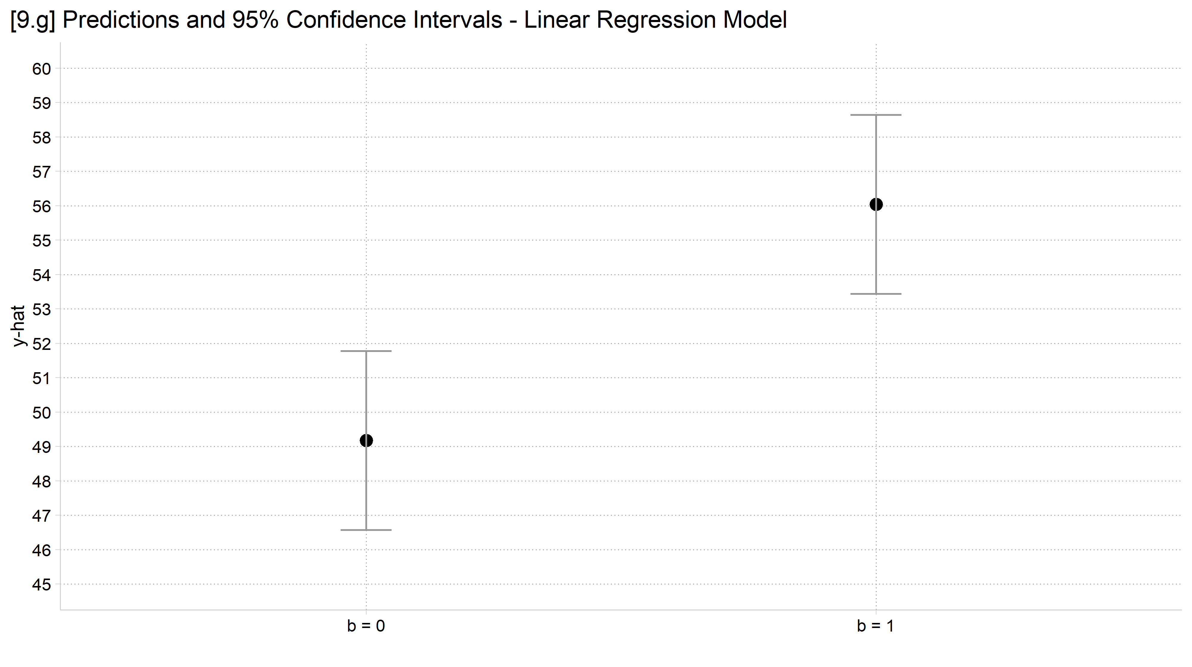
[9.g] Predicted y and 95% confidence intervals for b = 0 and b = 1: the two confidence intervals do not overlap.

// 9.h - Error term has SD of 20
est restore pr_y20
(results pr_y20 are active now)
coefplot, vertical ciop(recast(rcap) col(gs10)) ylab(45(1)60) ///
    xlab(1 "b = 0" 2 "b = 1") ytitle("y-hat") ///
    title("[9.h] Predictions and 95% Confidence Intervals - Linear Regression 
Model")

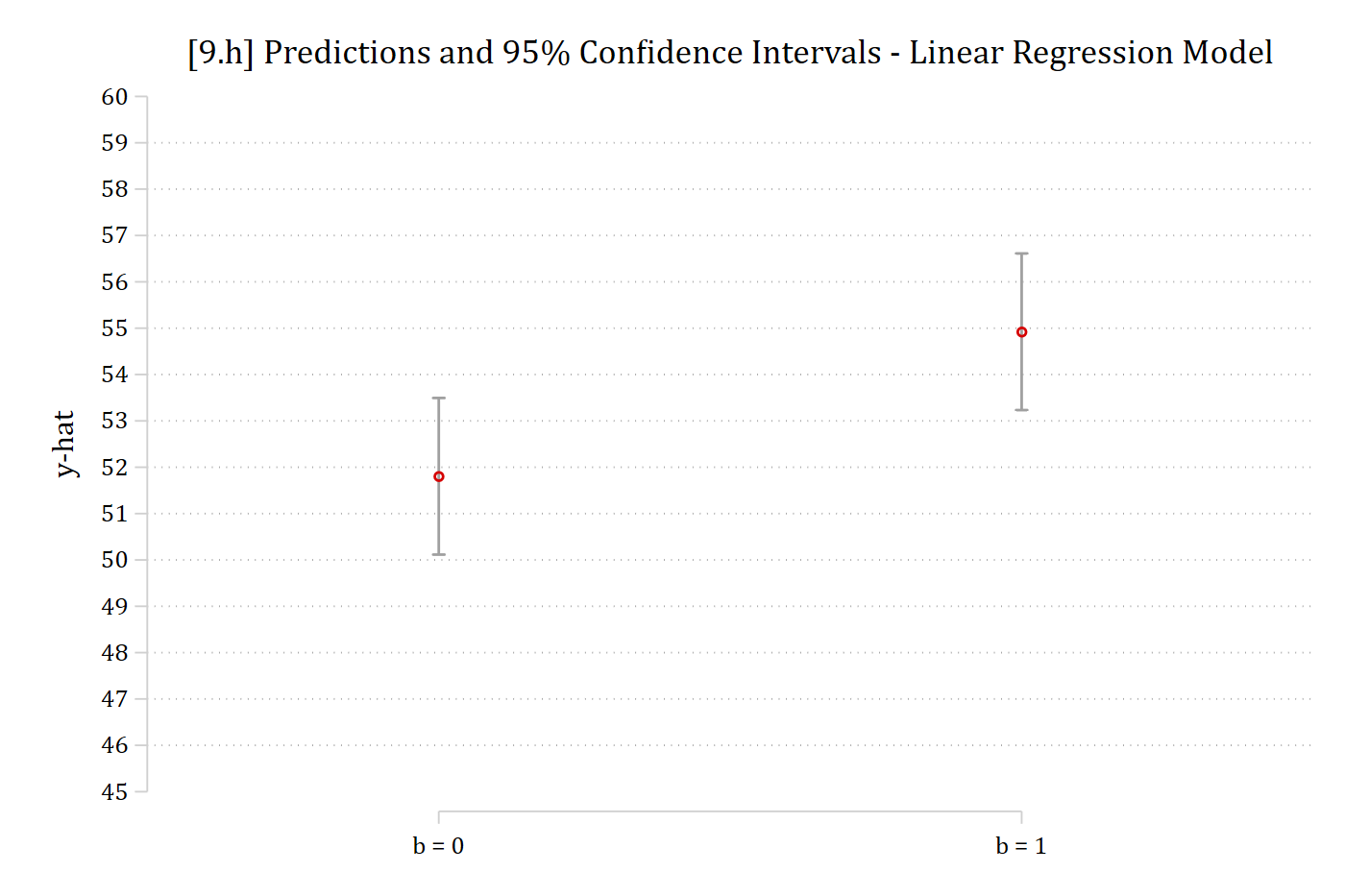
[9.h] Predicted y and 95% confidence intervals for b = 0 (about 51.8) and b = 1 (about 54.9): the confidence intervals overlap slightly.

# 9.h - Error term has SD of 20
ci_plot("y20", "9.h")

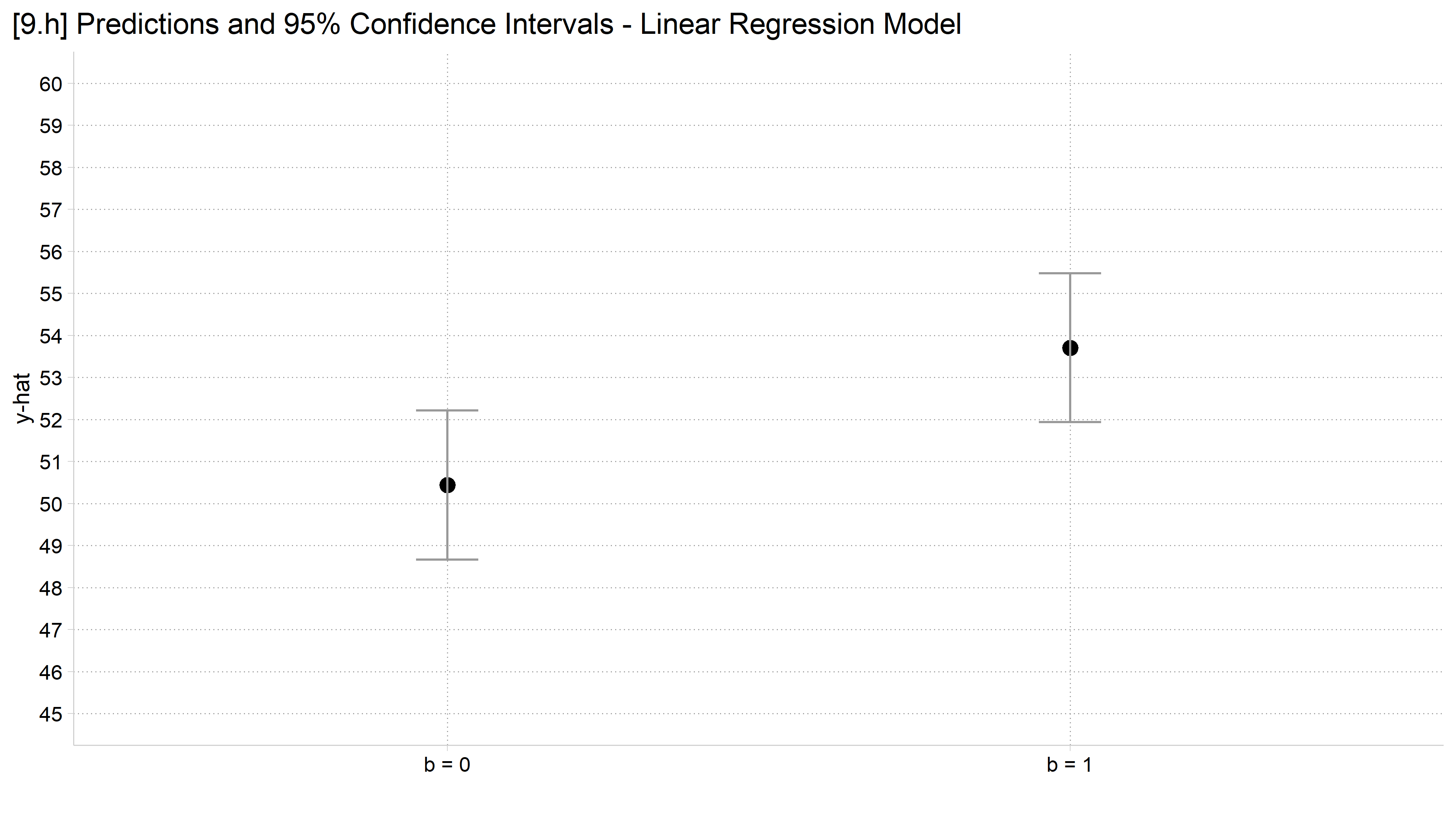
[9.h] Predicted y and 95% confidence intervals for b = 0 and b = 1: the confidence intervals overlap slightly.

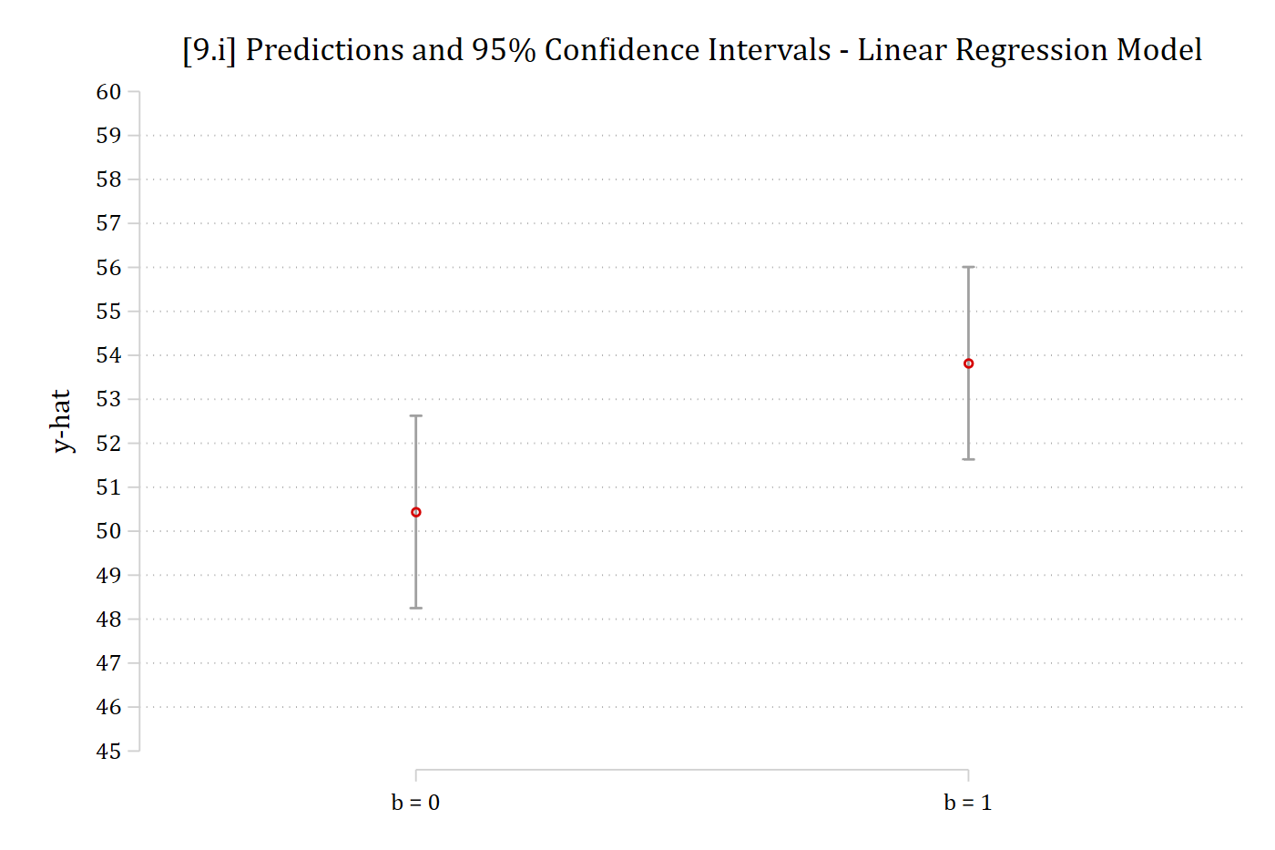
// 9.i - Error term has SD of 25
est restore pr_y25
(results pr_y25 are active now)
coefplot, vertical ciop(recast(rcap) col(gs10)) ylab(45(1)60) ///
    xlab(1 "b = 0" 2 "b = 1") ytitle("y-hat") ///
    title("[9.i] Predictions and 95% Confidence Intervals - Linear Regression 
Model")

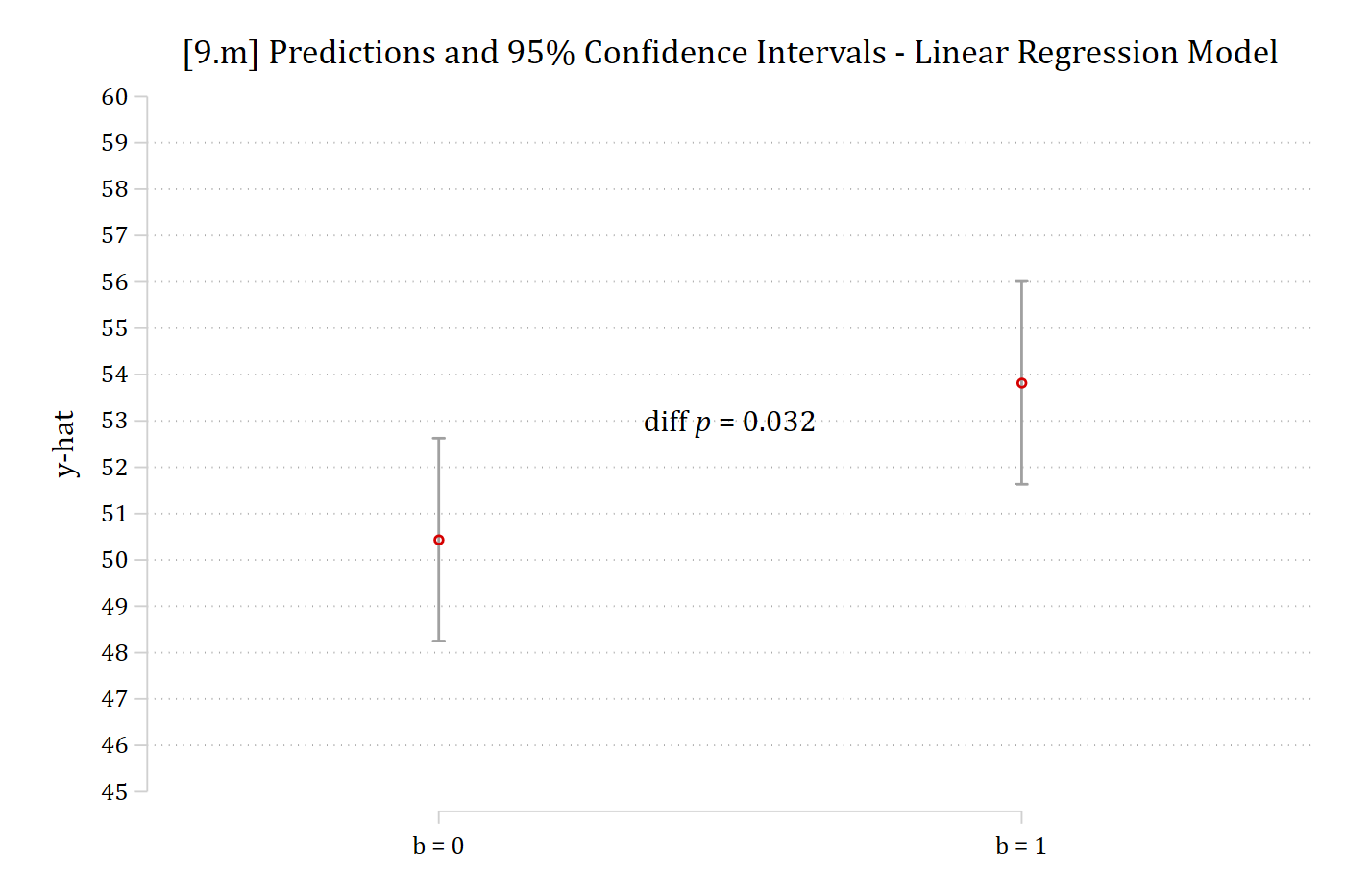
[9.i] Predicted y and 95% confidence intervals for b = 0 (about 50.4) and b = 1 (about 53.8): the confidence intervals overlap by about a point.

# 9.i - Error term has SD of 25
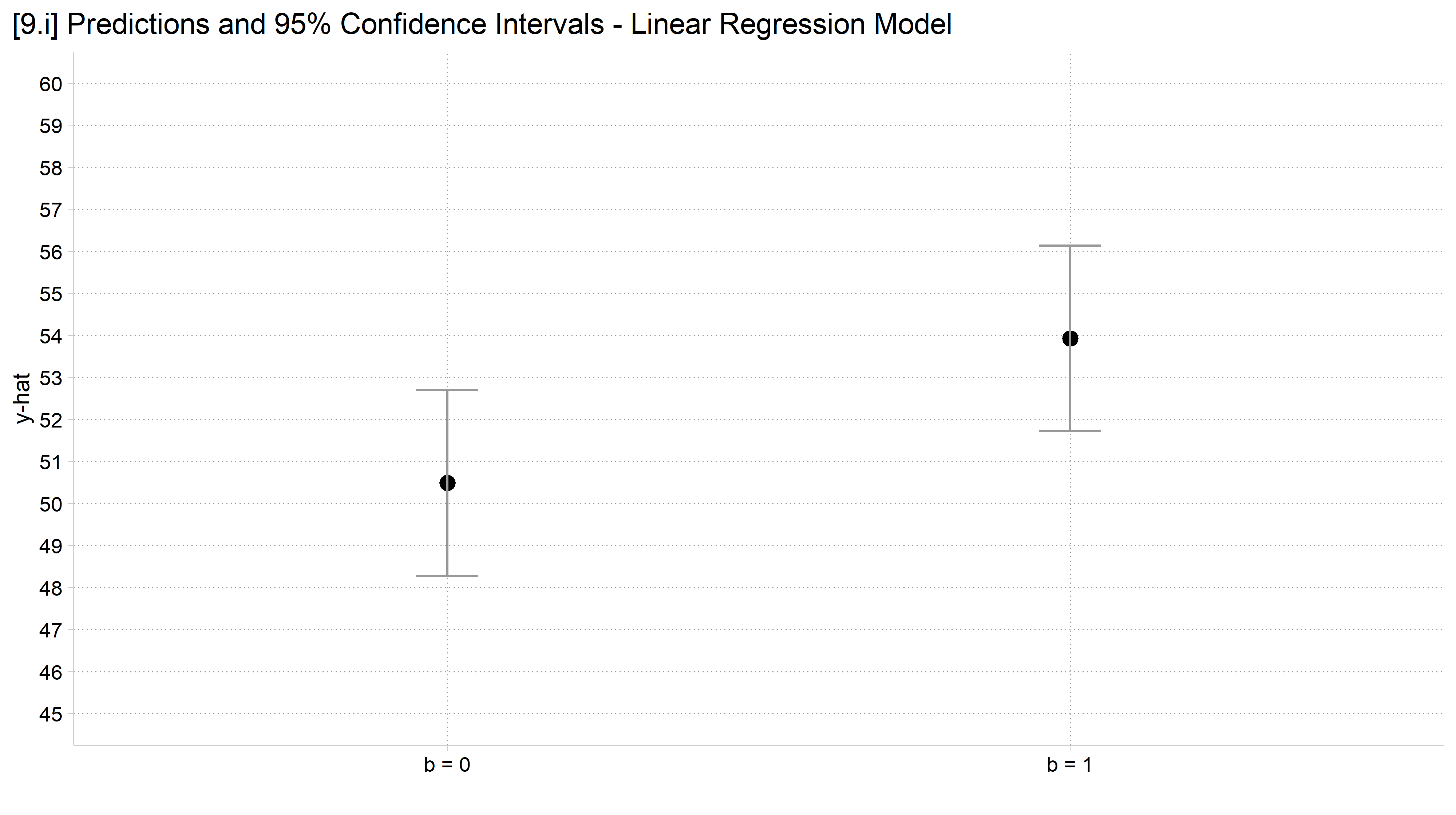
ci_plot("y25", "9.i")

[9.i] Predicted y and 95% confidence intervals for b = 0 and b = 1: the confidence intervals overlap by about a point.

With the significance tests

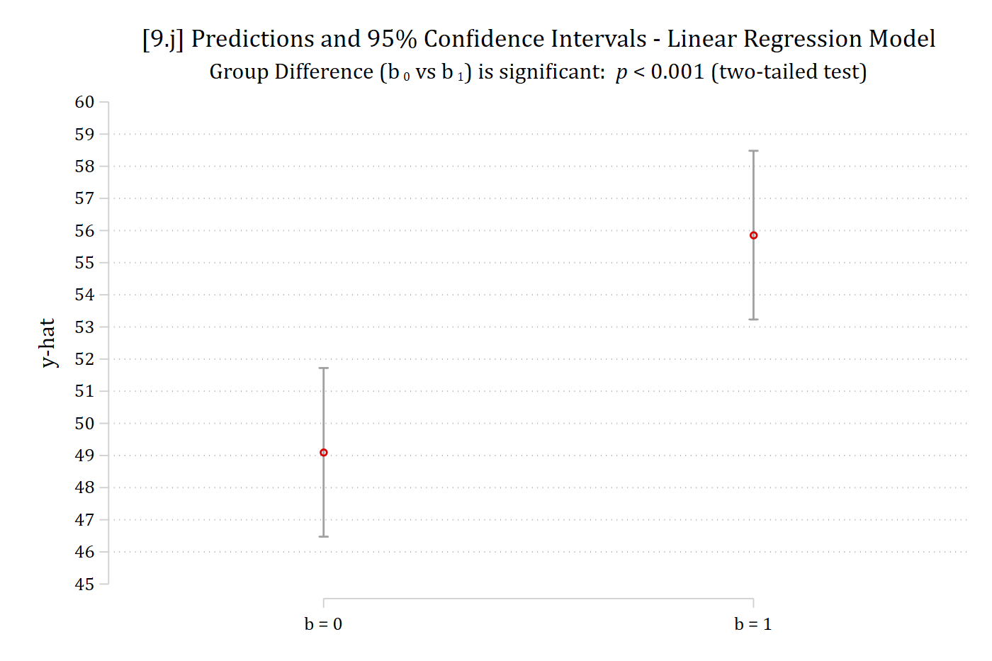
// 9.j - Error term has SD of 30
est restore pr_y30
(results pr_y30 are active now)
lincom 2._at - 1._at    // test of the difference in predictions
 ( 1)  - 1bn._at + 2._at = 0

------------------------------------------------------------------------------
             | Coefficient  Std. err.      t    P>|t|     [95% conf. interval]
-------------+----------------------------------------------------------------
         (1) |      6.758      1.891    3.574   0.000        3.047      10.469
------------------------------------------------------------------------------
coefplot, vertical ciop(recast(rcap) col(gs10)) ylab(45(1)60) ///
    xlab(1 "b = 0" 2 "b = 1") ytitle("y-hat") ///
    title("[9.j] Predictions and 95% Confidence Intervals - Linear Regression 
Model") ///
    subtitle("Group Difference (b{sub: 0} vs b{sub: 1}) is significant: {it: p
} < 0.001 (two-tailed test)")

[9.j] The SD 30 predictions again, with the subtitle: Group difference (b0 vs b1) is significant, p < 0.001 (two-tailed test).

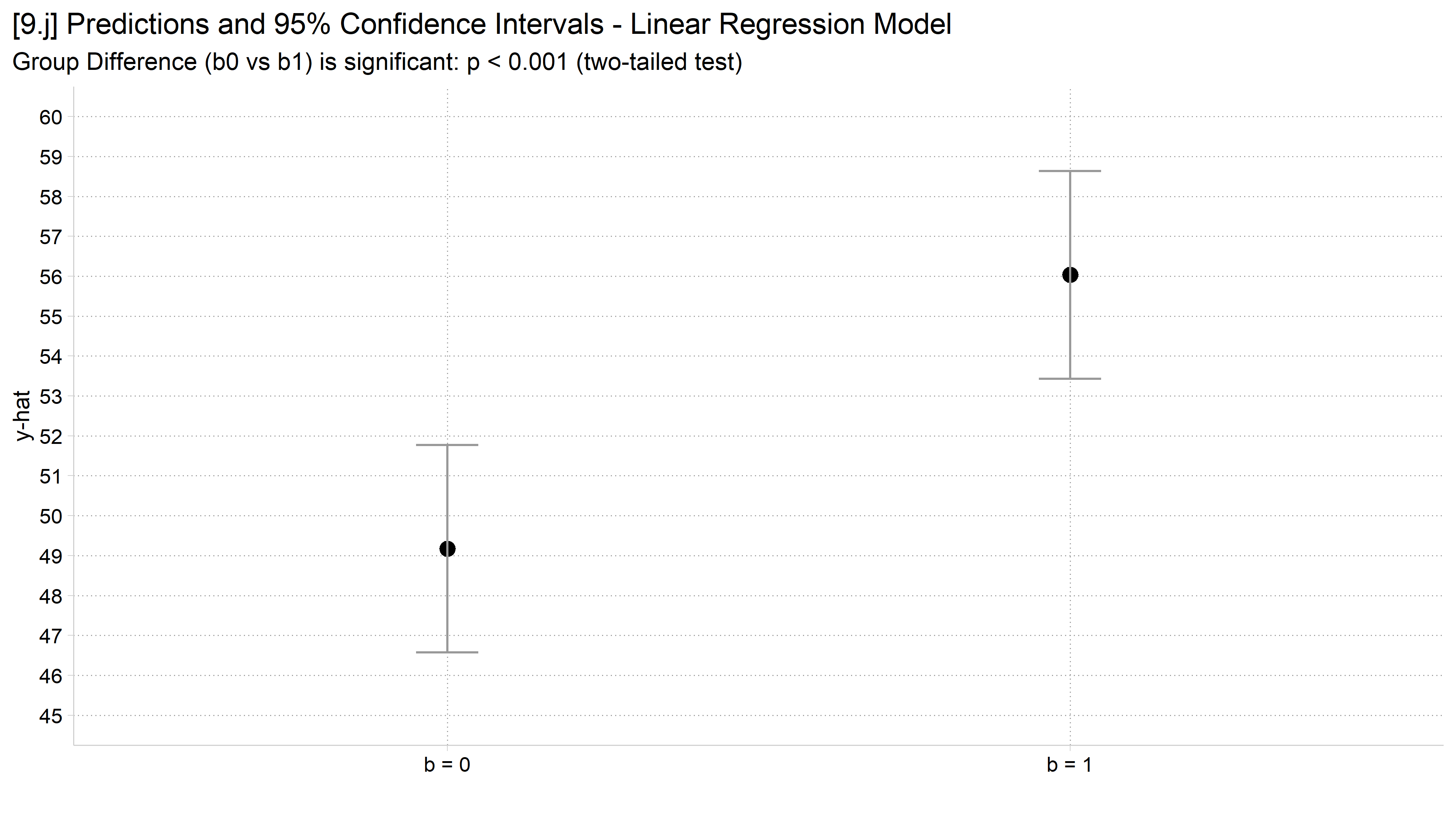
# 9.j - Error term has SD of 30
avg_comparisons(lm(y30 ~ b, data = sim), variables = "b")

 Estimate Std. Error    z Pr(>|z|)    S 2.5 % 97.5 %
     6.86       1.88 3.66   <0.001 11.9  3.18   10.5

Term: b
Type: response
Comparison: 1 - 0
ci_plot("y30", "9.j", show_p = TRUE)

[9.j] The SD 30 predictions again, with the subtitle: Group difference (b0 vs b1) is significant, p < 0.001 (two-tailed test).

// 9.k - Error term has SD of 20
est restore pr_y20
(results pr_y20 are active now)
lincom 2._at - 1._at    // test of the difference in predictions
 ( 1)  - 1bn._at + 2._at = 0

------------------------------------------------------------------------------
             | Coefficient  Std. err.      t    P>|t|     [95% conf. interval]
-------------+----------------------------------------------------------------
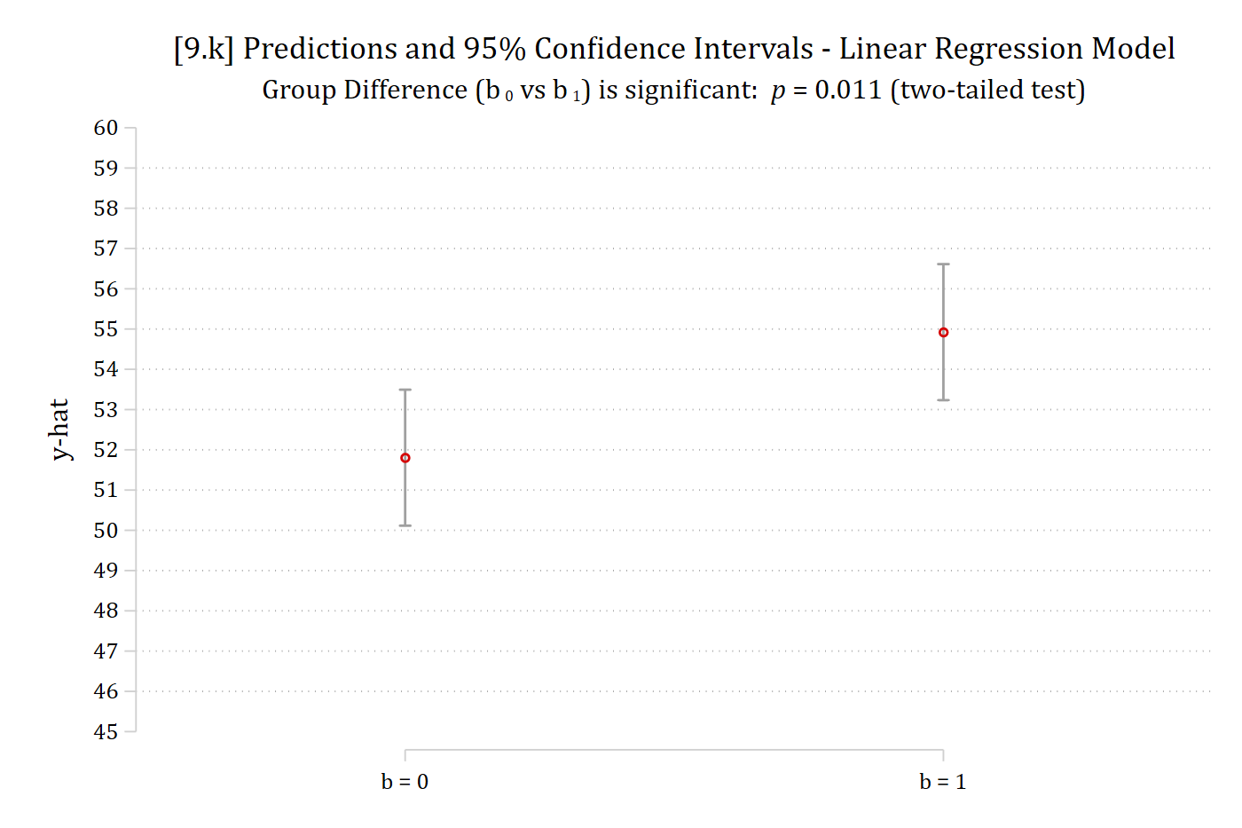
         (1) |      3.118      1.218    2.561   0.011        0.729       5.507
------------------------------------------------------------------------------
coefplot, vertical ciop(recast(rcap) col(gs10)) ylab(45(1)60) ///
    xlab(1 "b = 0" 2 "b = 1") ytitle("y-hat") ///
    title("[9.k] Predictions and 95% Confidence Intervals - Linear Regression 
Model") ///
    subtitle("Group Difference (b{sub: 0} vs b{sub: 1}) is significant: {it: p
} = 0.011 (two-tailed test)")

[9.k] The SD 20 predictions again, whose confidence intervals overlap slightly, with the subtitle: Group difference (b0 vs b1) is significant, p = 0.011 (two-tailed test).

# 9.k - Error term has SD of 20
avg_comparisons(lm(y20 ~ b, data = sim), variables = "b")

 Estimate Std. Error    z Pr(>|z|)   S 2.5 % 97.5 %
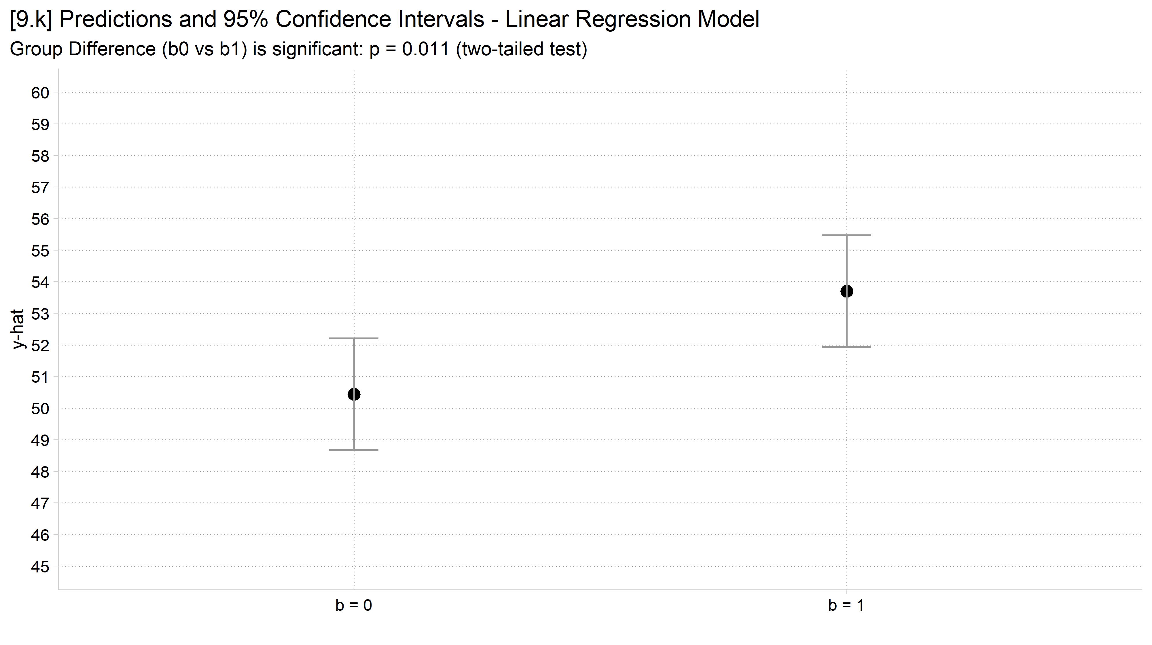
     3.27       1.28 2.55   0.0106 6.6 0.761   5.77

Term: b
Type: response
Comparison: 1 - 0
ci_plot("y20", "9.k", show_p = TRUE)

[9.k] The SD 20 predictions again, whose confidence intervals overlap slightly, with the subtitle saying the group difference is significant.

// 9.l - Error term has SD of 25
est restore pr_y25
(results pr_y25 are active now)
lincom 2._at - 1._at    // test of the difference in predictions
 ( 1)  - 1bn._at + 2._at = 0

------------------------------------------------------------------------------
             | Coefficient  Std. err.      t    P>|t|     [95% conf. interval]
-------------+----------------------------------------------------------------
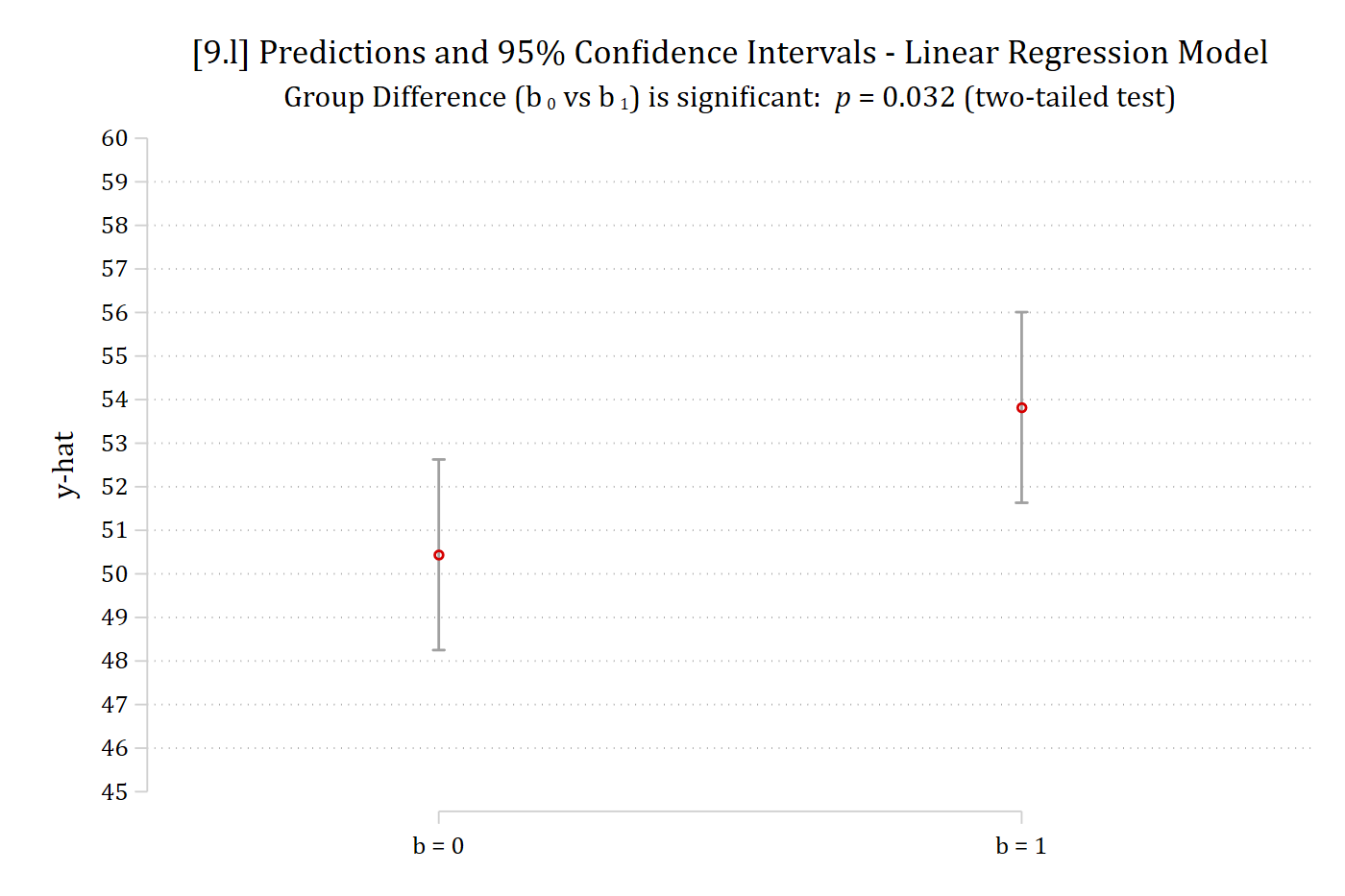
         (1) |      3.382      1.577    2.145   0.032        0.288       6.476
------------------------------------------------------------------------------
coefplot, vertical ciop(recast(rcap) col(gs10)) ylab(45(1)60) ///
    xlab(1 "b = 0" 2 "b = 1") ytitle("y-hat") ///
    title("[9.l] Predictions and 95% Confidence Intervals - Linear Regression 
Model") ///
    subtitle("Group Difference (b{sub: 0} vs b{sub: 1}) is significant: {it: p
} = 0.032 (two-tailed test)")

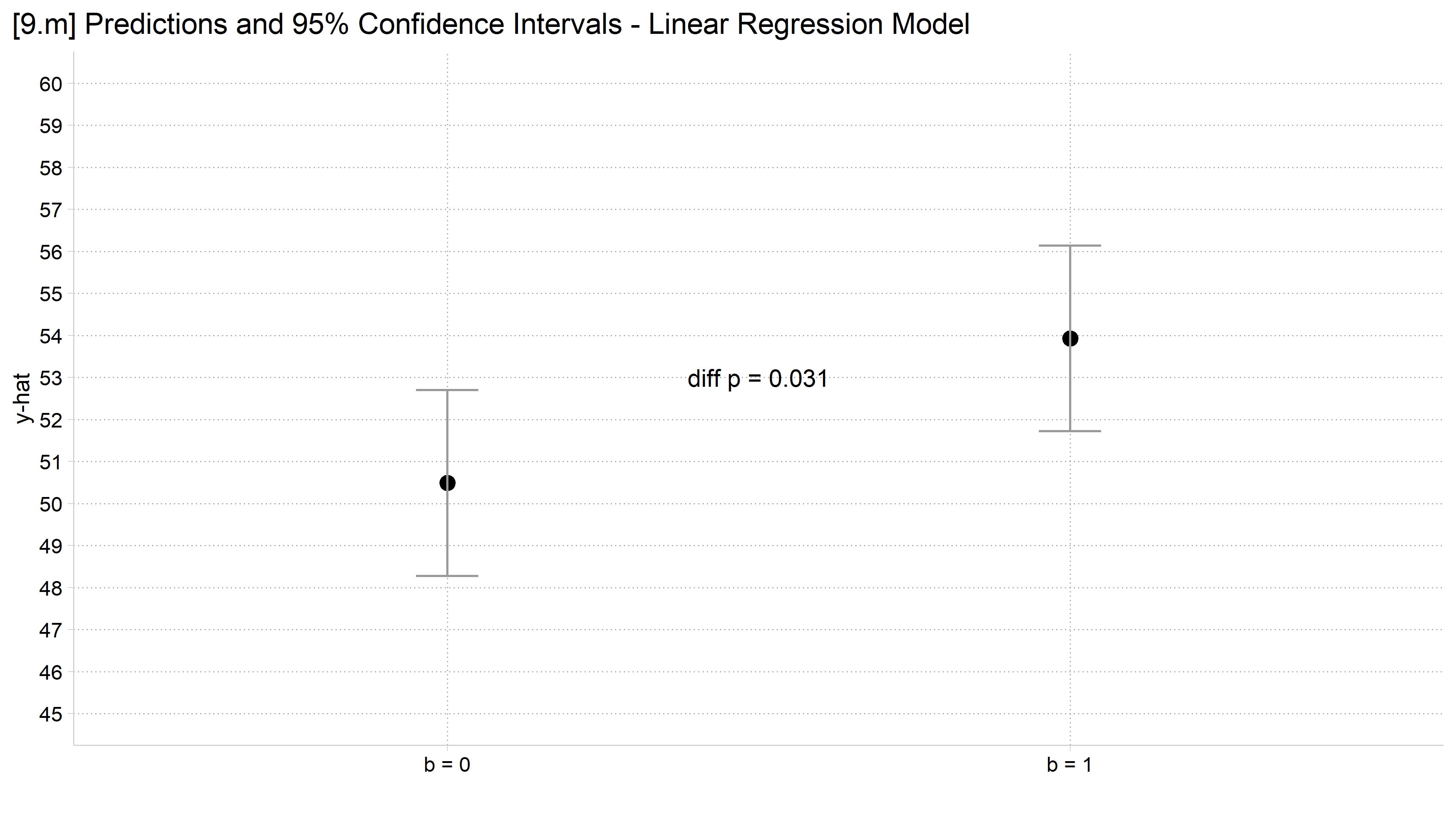
[9.l] The SD 25 predictions again, whose confidence intervals overlap, with the subtitle: Group difference (b0 vs b1) is significant, p = 0.032 (two-tailed test).

# 9.l - Error term has SD of 25
avg_comparisons(lm(y25 ~ b, data = sim), variables = "b")

 Estimate Std. Error    z Pr(>|z|)   S 2.5 % 97.5 %
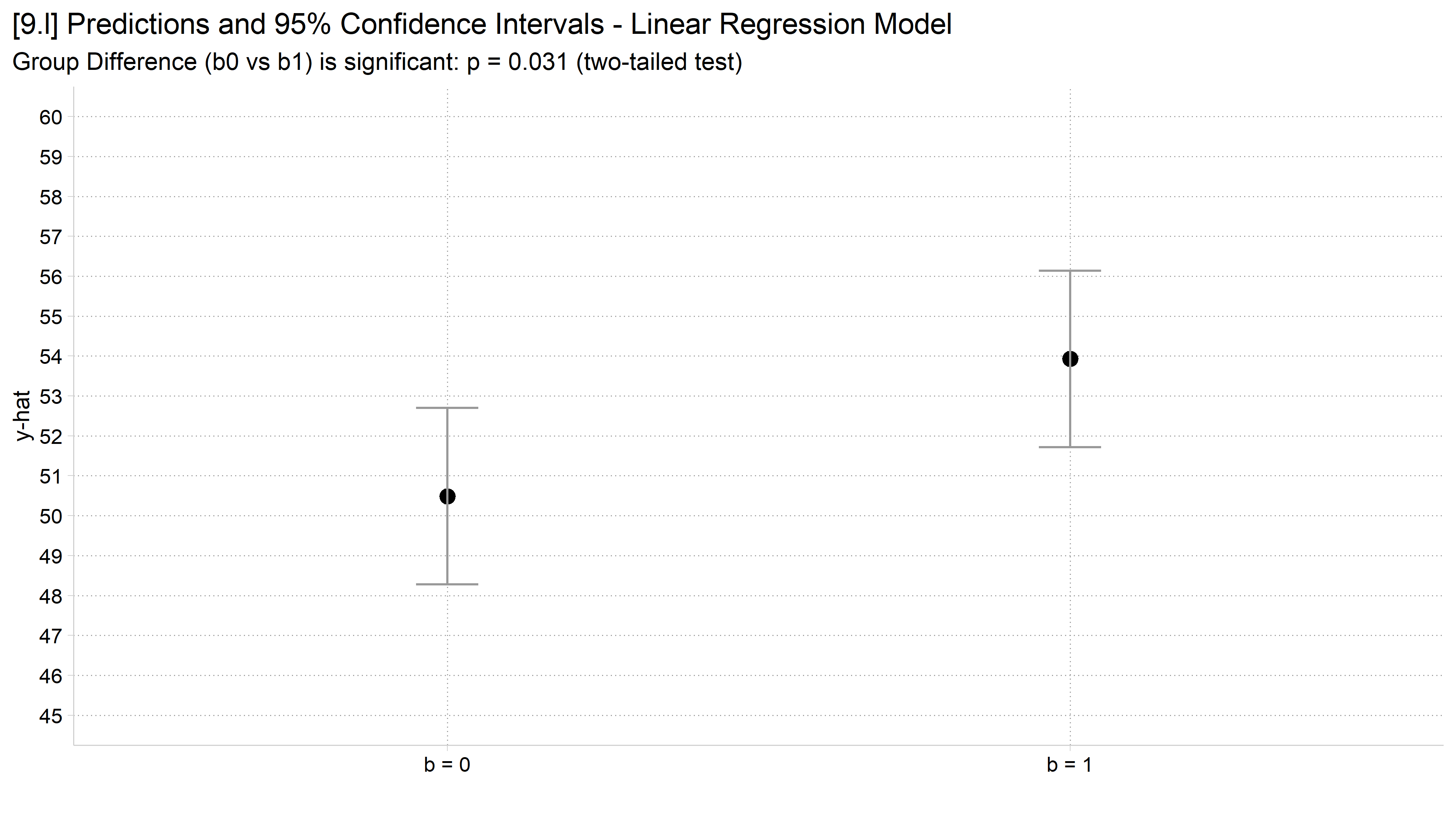
     3.44        1.6 2.16    0.031 5.0 0.315   6.57

Term: b
Type: response
Comparison: 1 - 0
ci_plot("y25", "9.l", show_p = TRUE)

[9.l] The SD 25 predictions again, whose confidence intervals overlap, with the subtitle saying the group difference is significant.

Advice on confidence intervals and standard errors

  • Most people—including PhD researchers—do not understand what overlapping confidence intervals indicate about statistical significance
    • You need to recognize this when making graphics to present your findings
  • Importantly, when confidence intervals do not overlap (e.g., on the 1st plot above) this indicates that the group difference (i.e., b0 vs b1) is significant
    • However, when the confidence interval does overlap this may or may not indicate the group difference is non-significant*: you must test for this directly. As Belia et al. (2005) gently put it:

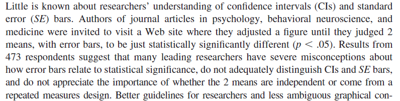
Excerpt from the Belia et al. (2005) abstract: little is known about researchers' understanding of confidence intervals and standard error bars, and many leading researchers have severe misconceptions about how error bars relate to statistical significance.

// 9.m - Add significance info to the graph using the text( ) option
*NOTE: specify the y-x coordinates for where to place text
coefplot, vertical ciop(recast(rcap) col(gs10)) ylab(45(1)60) ///
    xlab(1 "b = 0" 2 "b = 1") ytitle("y-hat") ///
    title("[9.m] Predictions and 95% Confidence Intervals - Linear Regression 
Model") ///
    text(53 1.5 "diff {it:p} = 0.032")

[9.m] The SD 25 predictions with the text diff p = 0.032 placed on the graph between the two groups.

# 9.m - Add the significance test of the difference to the graph itself
m25 <- lm(y25 ~ b, data = sim)
p25 <- avg_comparisons(m25, variables = "b")$p.value
ci_plot("y25", "9.m") +
  annotate("text", x = 1.5, y = 53, label = paste0("diff p = ", round(p25, 3)))
[9.m] The SD 25 predictions with the p-value of the difference placed on the graph between the two groups.

Back to top