3.0 Binary DVs and the Linear Probability Model

Expectations for binary DVs

  • As with any regression, expectations (means) are being modeled

\[E(y\,|\,\mathbf{x}) = \Pr(y = 1\,|\,\mathbf{x})\]

  • With a binary DV coded 0/1, the mean is the proportion of 1’s observed
  • If DV is whether someone voted in the 2024 presidential election
    • In 2024, ≈65% of eligible U.S. voters voted. Consider probabilities of observing the binary values 0 (did not vote) and 1 (did vote):
y-value Proportion Observed Probability of Response
0 0.35 0.35
1 0.65 0.65
  • Usually, interested in expectations conditional on values of other variables
    • E.g., What if 70% of Republicans voted and only 60% non-Republicans voted?

\[E(y\,|\,x_{Republican} = 0) = \Pr(y = 1\,|\,x_{Republican} = 0) = 0.60\]

\[E(y\,|\,x_{Republican} = 1) = \Pr(y = 1\,|\,x_{Republican} = 1) = 0.70\]

Why not use a linear model for binary DVs?

  • When linear regression (usually estimated via OLS) is used for a binary DV this is referred to as the linear probability model (LPM)

\[E(y_{i}\,|\,\mathbf{x}) = \Pr(y_{i} = 1\,|\,\mathbf{x}) = \beta_{0} + \beta_{1}x_{i1} + \beta_{2}x_{i2} + \beta_{3}x_{i3}\]

  • Example
    • 2020 presidential voting intentions: Trump = 1; Not Trump = 0
      • NOTE: Including IVs for age, income, gender, sexuality, race-ethnicity, education, religiosity, etc.

\[{presvote}_{i} = \beta_{0} + \beta_{woman}{woman}_{i} + \beta_{educ}{educ}_{i} + \beta_{race}{race}_{i} \ldots\]

\[E({presvote}_{i}\,|\,\mathbf{x}) = \Pr({presvote}_{i} = 1\,|\,\mathbf{x}) = \beta_{0} + \beta_{woman}{woman}_{i} + \beta_{educ}{educ}_{i} + \beta_{race}{race}_{i} \ldots\]

  • The model is linear in the probability of y
use "https://tdmize.github.io/data/data/cda_anes", clear
(American National Election Study 2020 - Pre-election | CDA | 2021-09-26)
drop if missing(age, hhincome, woman, lgb, race4, ///
    edyrs, relimport, wrongtrack)
(948 observations deleted)
regress vote_trump age hhincome i.woman i.lgb i.race4 ///
    edyrs i.relimport i.wrongtrack
      Source |       SS           df       MS      Number of obs   =     6,857
-------------+----------------------------------   F(13, 6843)     =    412.52
       Model |  732.610452        13  56.3546502   Prob > F        =    0.0000
    Residual |  934.837411     6,843  .136612218   R-squared       =    0.4394
-------------+----------------------------------   Adj R-squared   =    0.4383
       Total |  1667.44786     6,856  .243210015   Root MSE        =    .36961

-------------------------------------------------------------------------------
   vote_trump | Coefficient  Std. err.      t    P>|t|     [95% conf. interval]
--------------+----------------------------------------------------------------
          age |     -0.001      0.000   -2.154   0.031       -0.001      -0.000
     hhincome |     -0.000      0.000   -0.812   0.417       -0.000       0.000
              |
        woman |
       Woman  |     -0.049      0.009   -5.364   0.000       -0.066      -0.031
              |
          lgb |
         LGB  |     -0.129      0.018   -6.982   0.000       -0.165      -0.093
              |
        race4 |
       Black  |     -0.347      0.017  -21.015   0.000       -0.380      -0.315
    Hispanic  |     -0.162      0.016   -9.925   0.000       -0.194      -0.130
       Other  |     -0.089      0.016   -5.515   0.000       -0.121      -0.058
              |
        edyrs |     -0.019      0.002   -9.766   0.000       -0.023      -0.015
              |
    relimport |
2. Very im..  |     -0.085      0.013   -6.332   0.000       -0.111      -0.059
3. Moderat..  |     -0.138      0.013  -10.243   0.000       -0.164      -0.112
4. A littl..  |     -0.183      0.016  -11.816   0.000       -0.214      -0.153
5. Not imp..  |     -0.285      0.014  -20.537   0.000       -0.312      -0.258
              |
   wrongtrack |
 Wrong track  |     -0.561      0.011  -52.030   0.000       -0.583      -0.540
        _cons |      1.368      0.033   41.483   0.000        1.303       1.433
-------------------------------------------------------------------------------
library(haven)           # import Stata data and labels
library(dplyr)           # data manipulation
library(ggplot2)         # graphs
library(marginaleffects) # predictions and marginal effects
library(cleanplots)      # graph scheme
cleanplots_defaults()

anes <- read_dta("https://tdmize.github.io/data/data/cda_anes.dta")

# Drop any missing data on the model IVs
anes <- anes[complete.cases(anes[c("age", "hhincome", "woman", "lgb", "race4",
  "edyrs", "relimport", "wrongtrack")]), ]

# Treat binary/nominal variables as factors using their value labels
anes <- anes |>
  mutate(woman = as_factor(woman), lgb = as_factor(lgb), race4 = as_factor(race4),
    relimport = as_factor(relimport), wrongtrack = as_factor(wrongtrack)) |>
  droplevels()

lpm1 <- lm(vote_trump ~ age + hhincome + woman + lgb + race4 + edyrs + relimport +
  wrongtrack, data = anes)
summary(lpm1)

Call:
lm(formula = vote_trump ~ age + hhincome + woman + lgb + race4 + 
    edyrs + relimport + wrongtrack, data = anes)

Residuals:
     Min       1Q   Median       3Q      Max 
-1.12431 -0.24707 -0.07862  0.13783  1.22325 

Coefficients:
                                   Estimate Std. Error t value Pr(>|t|)    
(Intercept)                       1.368e+00  3.298e-02  41.483  < 2e-16 ***
age                              -5.982e-04  2.777e-04  -2.154   0.0312 *  
hhincome                         -5.835e-05  7.184e-05  -0.812   0.4167    
womanWoman                       -4.863e-02  9.068e-03  -5.364 8.43e-08 ***
lgbLGB                           -1.287e-01  1.843e-02  -6.982 3.19e-12 ***
race4Black                       -3.474e-01  1.653e-02 -21.015  < 2e-16 ***
race4Hispanic                    -1.616e-01  1.629e-02  -9.925  < 2e-16 ***
race4Other                       -8.941e-02  1.621e-02  -5.515 3.62e-08 ***
edyrs                            -1.912e-02  1.958e-03  -9.766  < 2e-16 ***
relimport2. Very important       -8.496e-02  1.342e-02  -6.332 2.57e-10 ***
relimport3. Moderately important -1.379e-01  1.347e-02 -10.243  < 2e-16 ***
relimport4. A little important   -1.835e-01  1.553e-02 -11.816  < 2e-16 ***
relimport5. Not important at all -2.850e-01  1.388e-02 -20.537  < 2e-16 ***
wrongtrackWrong track            -5.615e-01  1.079e-02 -52.030  < 2e-16 ***
---
Signif. codes:  0 '***' 0.001 '**' 0.01 '*' 0.05 '.' 0.1 ' ' 1

Residual standard error: 0.3696 on 6843 degrees of freedom
  (475 observations deleted due to missingness)
Multiple R-squared:  0.4394,    Adjusted R-squared:  0.4383 
F-statistic: 412.5 on 13 and 6843 DF,  p-value: < 2.2e-16

Interpreting the linear probability model (LPM)

  • An advantage of the LPM is that the coefficients are in terms of probabilities; they are also additive effects
    • For binary IVs: Group (coded as 1 on xk) has a βk higher/lower probability of y (=1) than group (coded as 0 on xk)
    • For continuous IVs: A one unit increase in xk is associated with a βk increase/decrease in the probability of y (=1)

Black voters are about 34.7 percentage points less likely to vote for Trump than White voters

Women are about 4.9 percentage points less likely to vote for Trump

Each additional year of age decreases the probability of voting for Trump by .001

After controlling for other factors, household income is not related to intentions to vote for Trump

Interpretation Tip: Probabilities can be converted to percentage points by multiplying by 100. Note you should not say percent as this is usually used for a multiplicative effect, not a probability

Problems with the linear probability model

  • Heteroscedastic errors & non-normal errors
    • Standard errors, and thus p-values and CIs, will be incorrect
      • Using robust SEs can help
      • Whether they help enough to entirely fix the problem is unclear
  • King and Roberts (2015) argue convincingly that “…when misspecification is bad enough to make classical and robust standard errors diverge, assuming that it is nevertheless not so bad as to bias everything else requires considerable optimism. And even if the optimism is warranted, settling for a misspecified model, with or without robust standard errors, will still bias estimators of all but a few quantities of interest.”
    • In other words, using robust SEs does not “fix” the problem—instead, they are an indicator your model is wrong

Dr. Evil meme with the caption ROBUST.

  • Nonsensical predictions
    • Predictions outside the logical range of your DV
      • Binary DVs only take on the values of 0 or 1
      • Predicted probabilities can logically only range from 0 to 1
  • Measures of model fit (e.g. R2) are not interpretable
    • More on this later
  • Models tailor-made for binary DVs usually produce better model fit
  • Substantively unreasonable functional form
    • Want a functional form with reasonable nonlinearities built in that constrain predictions to a logical range
  • Unreasonable functional form often produces spurious interaction effects (Rohrer and Arslan 2021)

Linear probability model—single continuous IV

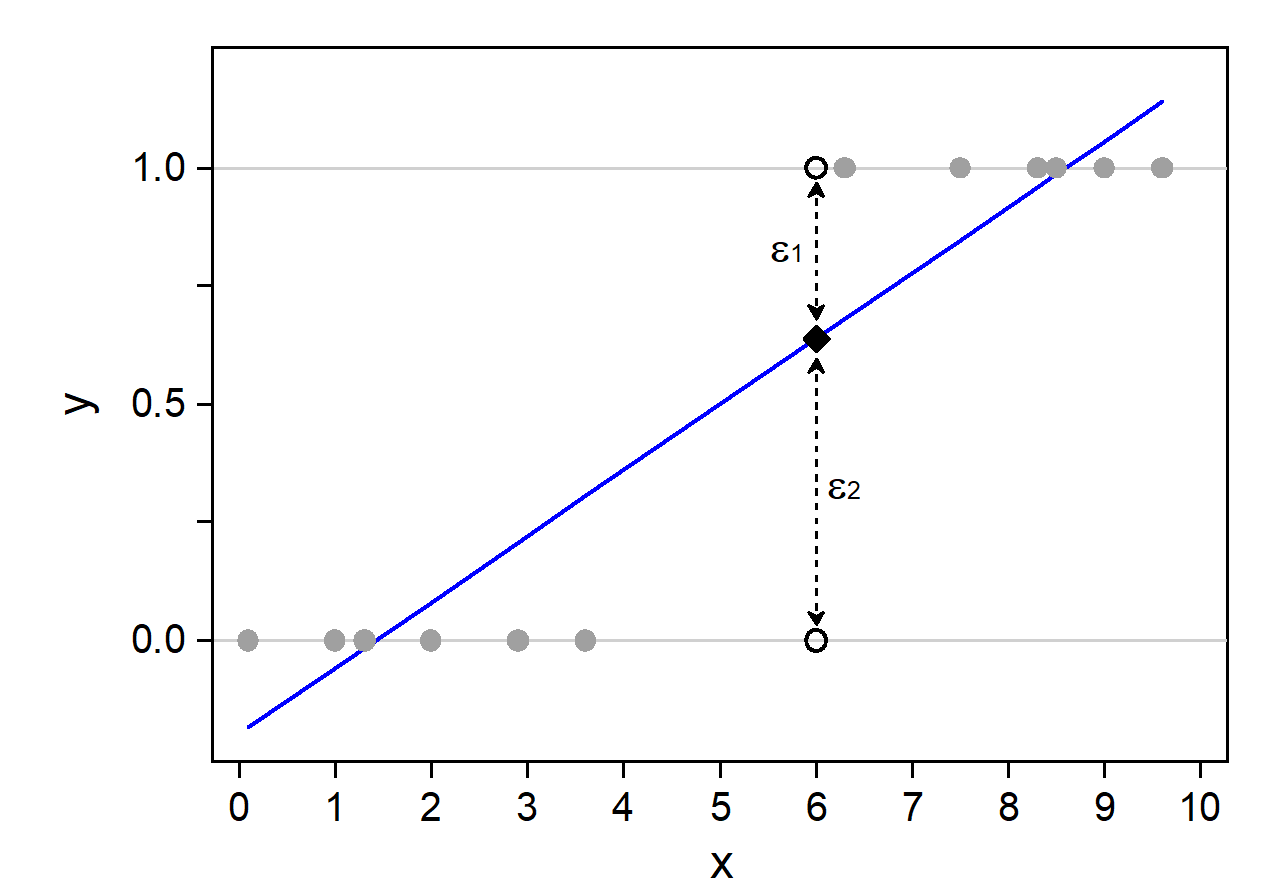
A straight LPM regression line through binary observations at y = 0 and y = 1: the line goes below 0 and above 1, and the errors at each x can only take two values.

Nonsensical predictions

  • According to the linear probability model (LPM)…
    • A highly-educated black woman has a predicted probability of voting for Trump of -.301
* Make prediction for highly educated black woman
mtable, at(woman=1 race4=2 edyrs=20 relimport=5 wrongtrack=1)
Expression: Linear prediction, predict()

      xb
--------
  -0.301

Specified values of covariates

           |    woman     race4     edyrs  relimport  wrongtrack
 ----------+----------------------------------------------------
   Current |        1         2        20          5           1
# Make prediction for highly educated black woman
avg_predictions(lpm1, newdata = datagrid(woman = "Woman", race4 = "Black", edyrs = 20,
  relimport = "5. Not important at all", wrongtrack = "Wrong track",
  grid_type = "counterfactual"))

 Estimate Std. Error   z Pr(>|z|)     S  2.5 % 97.5 %
   -0.301     0.0216 -14   <0.001 145.1 -0.344 -0.259

Type: response
  • A unit increase in xk results in a constant change βk in the probability
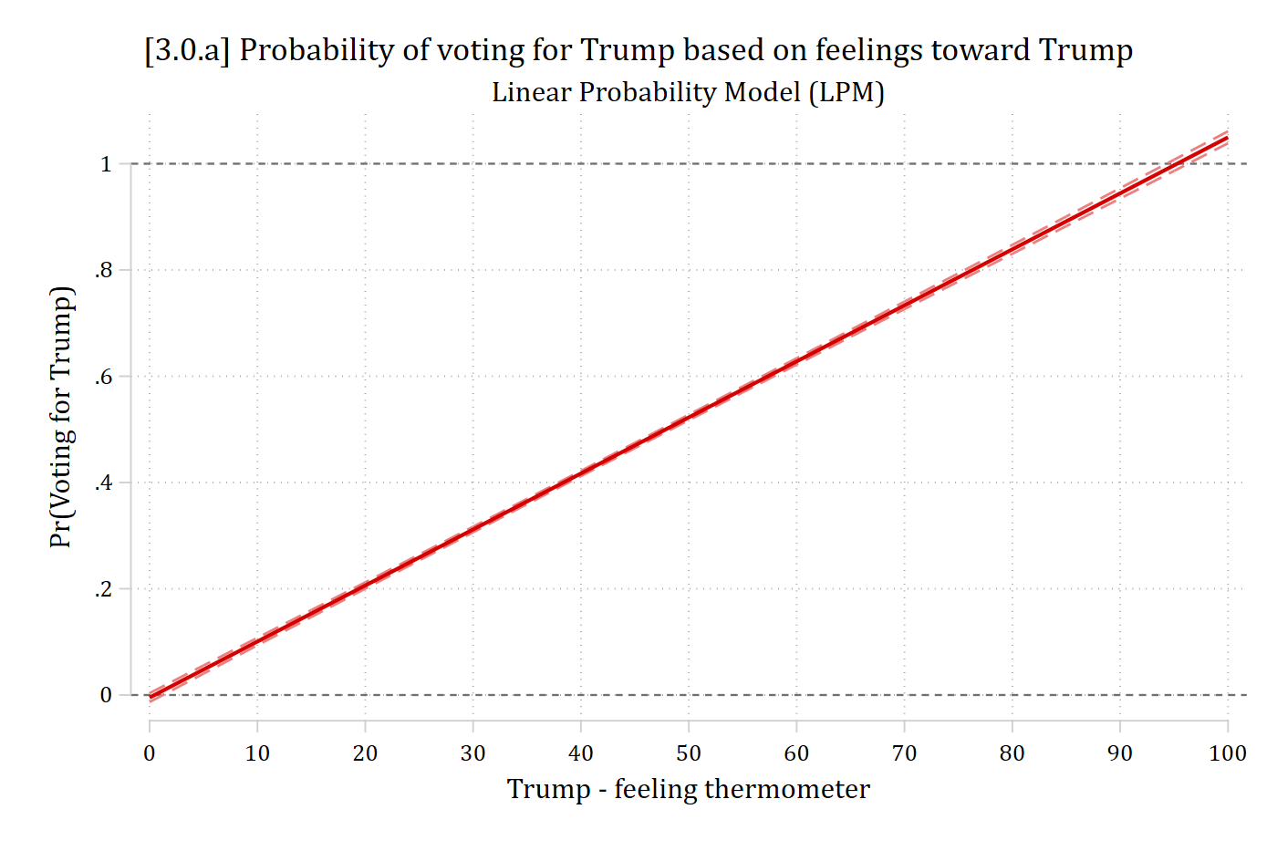
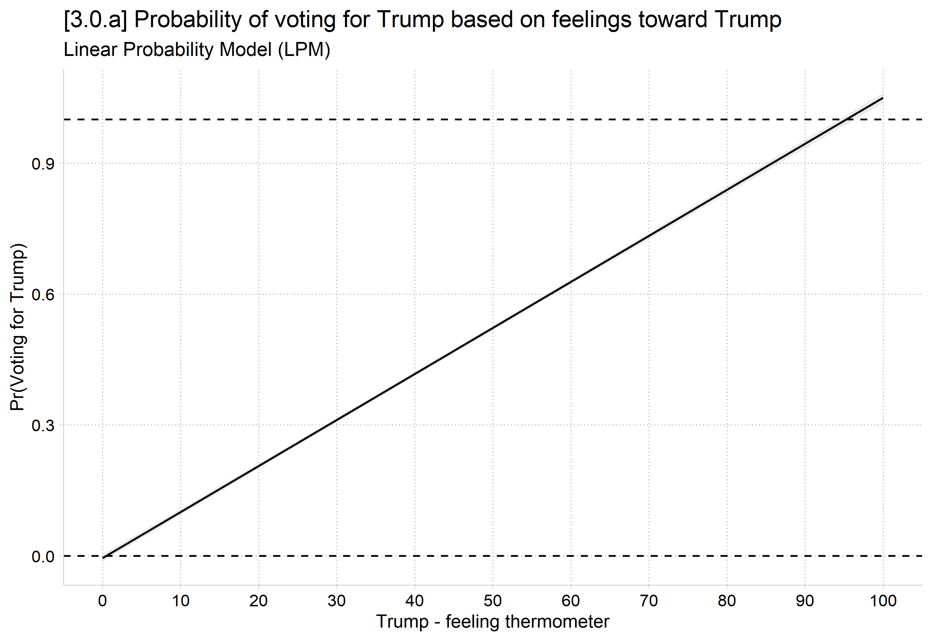
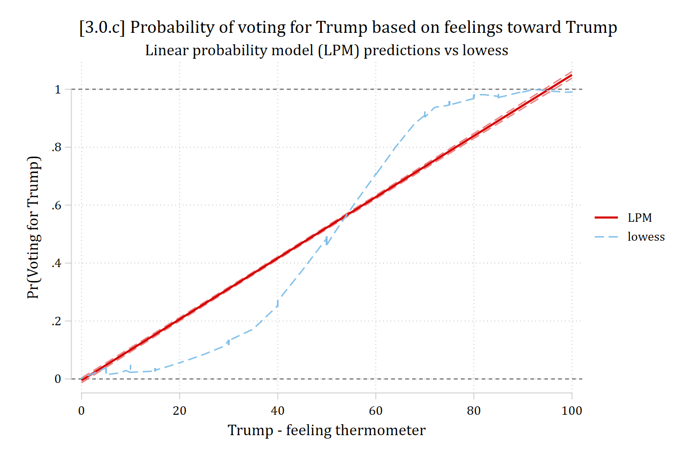
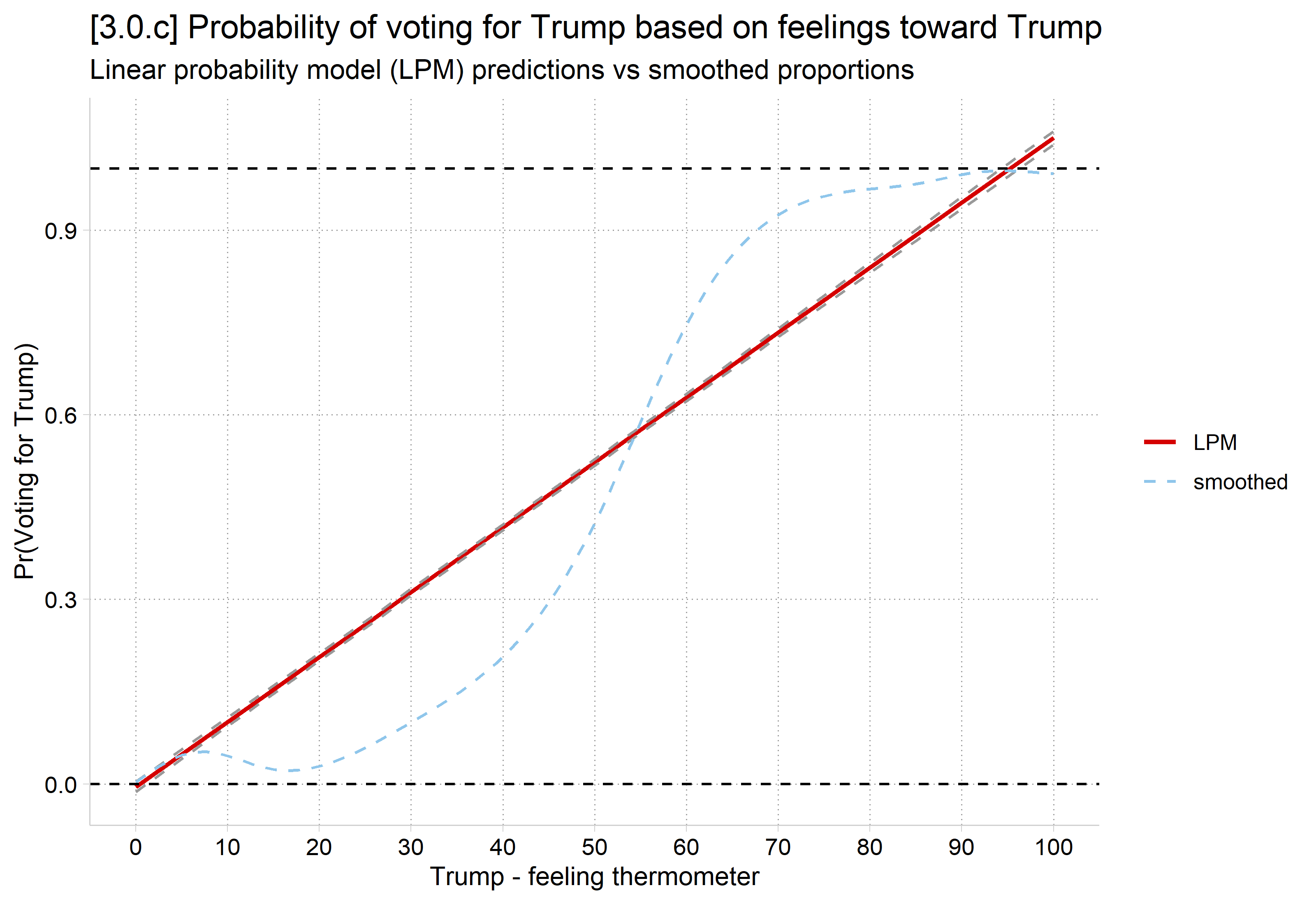
    • Substantively effects of feelings about Trump are likely to be diminishing
* Add Trump feeling thermometer to model
sum feel_trump, d
                 Trump - feeling thermometer
-------------------------------------------------------------
      Percentiles      Smallest
 1%            0              0
 5%            0              0
10%            0              0       Obs               7,155
25%            0              0       Sum of wgt.       7,155

50%           30                      Mean           39.65325
                        Largest       Std. dev.      40.26845
75%           85            100
90%          100            100       Variance       1621.548
95%          100            100       Skewness       .3315046
99%          100            100       Kurtosis       1.414096
regress vote_trump c.feel_trump age hhincome i.woman i.lgb i.race4 ///
    edyrs i.relimport i.wrongtrack
      Source |       SS           df       MS      Number of obs   =     6,695
-------------+----------------------------------   F(14, 6680)     =   2281.99
       Model |  1346.45847        14  96.1756049   Prob > F        =    0.0000
    Residual |  281.531673     6,680   .04214546   R-squared       =    0.8271
-------------+----------------------------------   Adj R-squared   =    0.8267
       Total |  1627.99014     6,694  .243201396   Root MSE        =    .20529

-------------------------------------------------------------------------------
   vote_trump | Coefficient  Std. err.      t    P>|t|     [95% conf. interval]
--------------+----------------------------------------------------------------
   feel_trump |      0.011      0.000  122.414   0.000        0.010       0.011
          age |     -0.000      0.000   -0.830   0.407       -0.000       0.000
     hhincome |      0.000      0.000    2.958   0.003        0.000       0.000
              |
        woman |
       Woman  |     -0.000      0.005   -0.013   0.989       -0.010       0.010
              |
          lgb |
         LGB  |     -0.019      0.010   -1.832   0.067       -0.039       0.001
              |
        race4 |
       Black  |     -0.082      0.010   -8.501   0.000       -0.100      -0.063
    Hispanic  |     -0.044      0.009   -4.794   0.000       -0.062      -0.026
       Other  |     -0.035      0.009   -3.847   0.000       -0.053      -0.017
              |
        edyrs |      0.002      0.001    1.417   0.157       -0.001       0.004
              |
    relimport |
2. Very im..  |     -0.009      0.008   -1.154   0.249       -0.024       0.006
3. Moderat..  |     -0.014      0.008   -1.895   0.058       -0.029       0.001
4. A littl..  |     -0.018      0.009   -2.067   0.039       -0.036      -0.001
5. Not imp..  |     -0.019      0.008   -2.391   0.017       -0.035      -0.003
              |
   wrongtrack |
 Wrong track  |     -0.030      0.007   -3.999   0.000       -0.044      -0.015
        _cons |      0.017      0.022    0.785   0.432       -0.025       0.059
-------------------------------------------------------------------------------
mtable, at(feel_trump=(0(10)100))
Expression: Linear prediction, predict()

           | feel_trump        xb
 ----------+---------------------
         1 |          0    -0.005
         2 |         10     0.101
         3 |         20     0.206
         4 |         30     0.312
         5 |         40     0.417
         6 |         50     0.522
         7 |         60     0.628
         8 |         70     0.733
         9 |         80     0.839
        10 |         90     0.944
        11 |        100     1.050

Specified values where .n indicates no values specified with at()

           |  No at()
 ----------+---------
   Current |       .n
# Add Trump feeling thermometer to model
summary(anes$feel_trump)
   Min. 1st Qu.  Median    Mean 3rd Qu.    Max.     NAs 
   0.00    0.00   30.00   39.65   85.00  100.00     177 
lpm2 <- lm(vote_trump ~ feel_trump + age + hhincome + woman + lgb + race4 + edyrs +
  relimport + wrongtrack, data = anes)
summary(lpm2)

Call:
lm(formula = vote_trump ~ feel_trump + age + hhincome + woman + 
    lgb + race4 + edyrs + relimport + wrongtrack, data = anes)

Residuals:
     Min       1Q   Median       3Q      Max 
-1.10290 -0.07148  0.00410  0.07333  1.06945 

Coefficients:
                                   Estimate Std. Error t value Pr(>|t|)    
(Intercept)                       1.692e-02  2.155e-02   0.785 0.432228    
feel_trump                        1.054e-02  8.614e-05 122.414  < 2e-16 ***
age                              -1.299e-04  1.566e-04  -0.830 0.406682    
hhincome                          1.197e-04  4.045e-05   2.958 0.003109 ** 
womanWoman                       -6.768e-05  5.113e-03  -0.013 0.989438    
lgbLGB                           -1.894e-02  1.034e-02  -1.832 0.066973 .  
race4Black                       -8.152e-02  9.589e-03  -8.501  < 2e-16 ***
race4Hispanic                    -4.412e-02  9.204e-03  -4.794 1.67e-06 ***
race4Other                       -3.517e-02  9.142e-03  -3.847 0.000121 ***
edyrs                             1.581e-03  1.116e-03   1.417 0.156584    
relimport2. Very important       -8.742e-03  7.576e-03  -1.154 0.248568    
relimport3. Moderately important -1.450e-02  7.652e-03  -1.895 0.058185 .  
relimport4. A little important   -1.826e-02  8.832e-03  -2.067 0.038769 *  
relimport5. Not important at all -1.933e-02  8.085e-03  -2.391 0.016836 *  
wrongtrackWrong track            -2.984e-02  7.461e-03  -3.999 6.43e-05 ***
---
Signif. codes:  0 '***' 0.001 '**' 0.01 '*' 0.05 '.' 0.1 ' ' 1

Residual standard error: 0.2053 on 6680 degrees of freedom
  (637 observations deleted due to missingness)
Multiple R-squared:  0.8271,    Adjusted R-squared:  0.8267 
F-statistic:  2282 on 14 and 6680 DF,  p-value: < 2.2e-16
avg_predictions(lpm2, by = "feel_trump",
  newdata = datagrid(feel_trump = seq(0, 100, 10), grid_type = "counterfactual"))

 feel_trump Estimate Std. Error      z Pr(>|z|)     S   2.5 %  97.5 %
          0 -0.00477    0.00426  -1.12    0.263   1.9 -0.0131 0.00358
         10  0.10068    0.00360  27.94   <0.001 568.1  0.0936 0.10774
         20  0.20613    0.00304  67.69   <0.001   Inf  0.2002 0.21209
         30  0.31158    0.00265 117.42   <0.001   Inf  0.3064 0.31678
         40  0.41703    0.00251 166.21   <0.001   Inf  0.4121 0.42194
         50  0.52248    0.00265 197.01   <0.001   Inf  0.5173 0.52767
         60  0.62792    0.00304 206.41   <0.001   Inf  0.6220 0.63389
         70  0.73337    0.00360 203.71   <0.001   Inf  0.7263 0.74043
         80  0.83882    0.00426 196.89   <0.001   Inf  0.8305 0.84717
         90  0.94427    0.00498 189.52   <0.001   Inf  0.9345 0.95404
        100  1.04972    0.00574 182.78   <0.001   Inf  1.0385 1.06098

Type: response

Note, observed range in data is 0 to 100 (\(\overline{x}\)=39.65)

margins, at(feel_trump=(0(5)100))
Predictive margins                                       Number of obs = 6,695
Model VCE: OLS

Expression: Linear prediction, predict()
1._at:  feel_trump =   0
2._at:  feel_trump =   5
3._at:  feel_trump =  10
4._at:  feel_trump =  15
5._at:  feel_trump =  20
6._at:  feel_trump =  25
7._at:  feel_trump =  30
8._at:  feel_trump =  35
9._at:  feel_trump =  40
10._at: feel_trump =  45
11._at: feel_trump =  50
12._at: feel_trump =  55
13._at: feel_trump =  60
14._at: feel_trump =  65
15._at: feel_trump =  70
16._at: feel_trump =  75
17._at: feel_trump =  80
18._at: feel_trump =  85
19._at: feel_trump =  90
20._at: feel_trump =  95
21._at: feel_trump = 100

------------------------------------------------------------------------------
             |            Delta-method
             |     Margin   std. err.      t    P>|t|     [95% conf. interval]
-------------+----------------------------------------------------------------
         _at |
          1  |     -0.005      0.004   -1.119   0.263       -0.013       0.004
          2  |      0.048      0.004   12.219   0.000        0.040       0.056
          3  |      0.101      0.004   27.938   0.000        0.094       0.108
          4  |      0.153      0.003   46.372   0.000        0.147       0.160
          5  |      0.206      0.003   67.694   0.000        0.200       0.212
          6  |      0.259      0.003   91.684   0.000        0.253       0.264
          7  |      0.312      0.003  117.418   0.000        0.306       0.317
          8  |      0.364      0.003  143.081   0.000        0.359       0.369
          9  |      0.417      0.003  166.212   0.000        0.412       0.422
         10  |      0.470      0.003  184.557   0.000        0.465       0.475
         11  |      0.522      0.003  197.015   0.000        0.517       0.528
         12  |      0.575      0.003  203.896   0.000        0.570       0.581
         13  |      0.628      0.003  206.407   0.000        0.622       0.634
         14  |      0.681      0.003  205.952   0.000        0.674       0.687
         15  |      0.733      0.004  203.709   0.000        0.726       0.740
         16  |      0.786      0.004  200.510   0.000        0.778       0.794
         17  |      0.839      0.004  196.889   0.000        0.830       0.847
         18  |      0.892      0.005  193.166   0.000        0.883       0.901
         19  |      0.944      0.005  189.519   0.000        0.935       0.954
         20  |      0.997      0.005  186.042   0.000        0.986       1.008
         21  |      1.050      0.006  182.779   0.000        1.038       1.061
------------------------------------------------------------------------------
marginsplot, ///
    xlab(0(10)100) ytitle("Pr(Voting for Trump)") yline(0 1) ///
    recastci(rline) ciopt(lpat(dash) color(*.5)) ///
    plotopt(msym(none) lwid(medthick)) ///
    title("[3.0.a] Probability of voting for Trump based on feelings toward Tr
ump", size(medium)) ///
    subtitle("Linear Probability Model (LPM)")
Variables that uniquely identify margins: feel_trump

LPM predicted probability of voting for Trump by the Trump feeling thermometer: a straight line rising from about 0 at 0 to above 1 at 100.

plot_predictions(lpm2, by = "feel_trump",
  newdata = datagrid(feel_trump = seq(0, 100, 5), grid_type = "counterfactual")) +
  geom_hline(yintercept = c(0, 1), linetype = "dashed") +
  scale_x_continuous(breaks = seq(0, 100, 10)) +
  labs(title = "[3.0.a] Probability of voting for Trump based on feelings toward Trump",
    subtitle = "Linear Probability Model (LPM)",
    x = "Trump - feeling thermometer", y = "Pr(Voting for Trump)")

LPM predicted probability of voting for Trump by the Trump feeling thermometer: a straight line rising from about 0 at 0 to above 1 at 100.

lowess vote_trump feel_trump, gen(lowpr) ///
    bwidth(0.15) ylab(#3) jitter(3) lineop(lwid(thick)) ///
    ytitle("Pr(voting for Trump)") xlab(0(10)100) ///
    title("[3.0.b] Smoothed proportion voting for Trump, by feelings toward Tr
ump (lowess)")

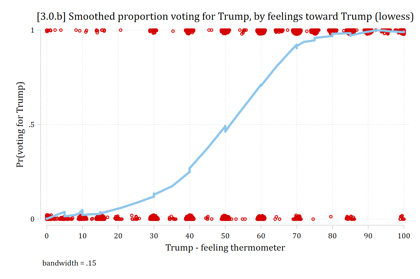
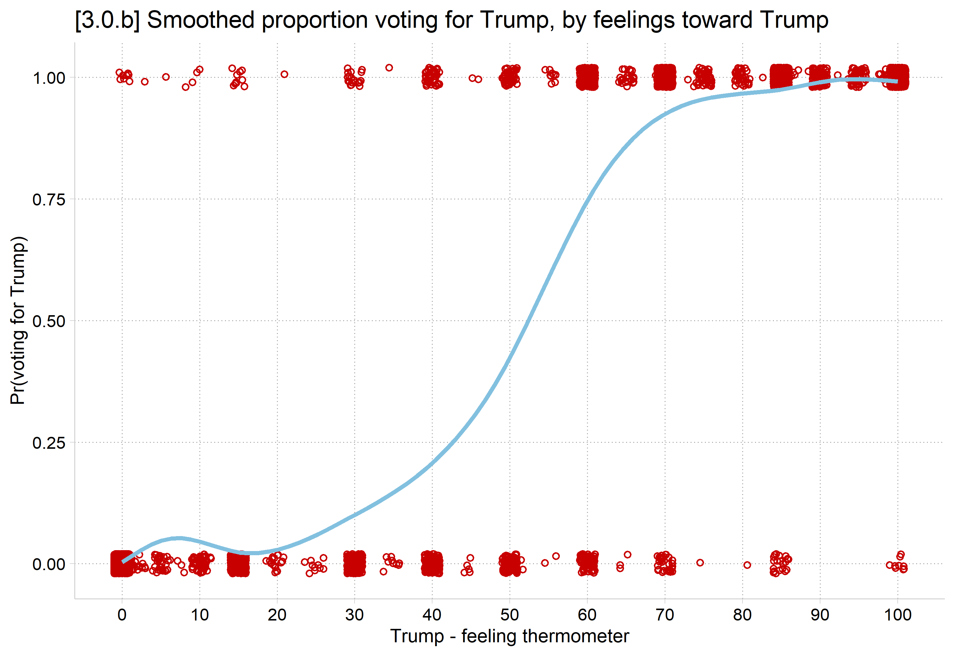
Lowess of voting for Trump by the Trump feeling thermometer over jittered observations at 0 and 1: an S-shaped curve that is flat near 0 at low feelings, rises steeply in the middle, and levels off near 1.

ggplot(anes, aes(x = feel_trump, y = vote_trump)) +
  geom_jitter(width = 1, height = 0.02, shape = 1, color = "#C80000") +
  geom_smooth(color = "#82C0DF", linewidth = 1.2, se = FALSE) +
  scale_x_continuous(breaks = seq(0, 100, 10)) +
  labs(title = "[3.0.b] Smoothed proportion voting for Trump, by feelings toward Trump",
    x = "Trump - feeling thermometer", y = "Pr(voting for Trump)")

Smoothed proportion voting for Trump by the Trump feeling thermometer over jittered observations at 0 and 1: an S-shaped curve that is flat near 0 at low feelings, rises steeply in the middle, and levels off near 1.

*Observed data: diminishing effects at each end of scale, and no values outside 0 to 1

margins, at(feel_trump=(0(5)100))
Predictive margins                                       Number of obs = 6,695
Model VCE: OLS

Expression: Linear prediction, predict()
1._at:  feel_trump =   0
2._at:  feel_trump =   5
3._at:  feel_trump =  10
4._at:  feel_trump =  15
5._at:  feel_trump =  20
6._at:  feel_trump =  25
7._at:  feel_trump =  30
8._at:  feel_trump =  35
9._at:  feel_trump =  40
10._at: feel_trump =  45
11._at: feel_trump =  50
12._at: feel_trump =  55
13._at: feel_trump =  60
14._at: feel_trump =  65
15._at: feel_trump =  70
16._at: feel_trump =  75
17._at: feel_trump =  80
18._at: feel_trump =  85
19._at: feel_trump =  90
20._at: feel_trump =  95
21._at: feel_trump = 100

------------------------------------------------------------------------------
             |            Delta-method
             |     Margin   std. err.      t    P>|t|     [95% conf. interval]
-------------+----------------------------------------------------------------
         _at |
          1  |     -0.005      0.004   -1.119   0.263       -0.013       0.004
          2  |      0.048      0.004   12.219   0.000        0.040       0.056
          3  |      0.101      0.004   27.938   0.000        0.094       0.108
          4  |      0.153      0.003   46.372   0.000        0.147       0.160
          5  |      0.206      0.003   67.694   0.000        0.200       0.212
          6  |      0.259      0.003   91.684   0.000        0.253       0.264
          7  |      0.312      0.003  117.418   0.000        0.306       0.317
          8  |      0.364      0.003  143.081   0.000        0.359       0.369
          9  |      0.417      0.003  166.212   0.000        0.412       0.422
         10  |      0.470      0.003  184.557   0.000        0.465       0.475
         11  |      0.522      0.003  197.015   0.000        0.517       0.528
         12  |      0.575      0.003  203.896   0.000        0.570       0.581
         13  |      0.628      0.003  206.407   0.000        0.622       0.634
         14  |      0.681      0.003  205.952   0.000        0.674       0.687
         15  |      0.733      0.004  203.709   0.000        0.726       0.740
         16  |      0.786      0.004  200.510   0.000        0.778       0.794
         17  |      0.839      0.004  196.889   0.000        0.830       0.847
         18  |      0.892      0.005  193.166   0.000        0.883       0.901
         19  |      0.944      0.005  189.519   0.000        0.935       0.954
         20  |      0.997      0.005  186.042   0.000        0.986       1.008
         21  |      1.050      0.006  182.779   0.000        1.038       1.061
------------------------------------------------------------------------------
marginsplot, ///
    xlab(0(10)100) ytitle("Pr(Voting for Trump)") yline(0 1) ///
    recastci(rline) ciopt(lpat(dash) color(*.5)) ///
    plotopt(msym(none) lwid(medthick)) ///
    title("[3.0.c] Probability of voting for Trump based on feelings toward Tr
ump", size(medium)) ///
    subtitle("Linear probability model (LPM) predictions vs lowess") ///
    addplot(connected lowpr feel_trump, sort msymbol(none) lcol(eltblue)) ///
    legend(order(2 "LPM" 3 "lowess"))
Variables that uniquely identify margins: feel_trump

LPM predictions and the lowess curve for voting for Trump by the Trump feeling thermometer: the straight LPM line is above the smoothed curve at low feelings, below it in the middle, and goes above 1 at the top.

lpm_prs <- avg_predictions(lpm2, by = "feel_trump",
  newdata = datagrid(feel_trump = seq(0, 100, 5), grid_type = "counterfactual"))

ggplot(lpm_prs, aes(x = feel_trump, y = estimate)) +
  geom_line(aes(color = "LPM"), linewidth = 1) +
  geom_line(aes(y = conf.low), linetype = "dashed", color = "gray60") +
  geom_line(aes(y = conf.high), linetype = "dashed", color = "gray60") +
  geom_smooth(data = anes, aes(x = feel_trump, y = vote_trump, color = "smoothed"),
    linetype = "dashed", se = FALSE) +
  geom_hline(yintercept = c(0, 1), linetype = "dashed") +
  scale_x_continuous(breaks = seq(0, 100, 10)) +
  labs(title = "[3.0.c] Probability of voting for Trump based on feelings toward Trump",
    subtitle = "Linear probability model (LPM) predictions vs smoothed proportions",
    x = "Trump - feeling thermometer", y = "Pr(Voting for Trump)", color = NULL)

LPM predictions and the smoothed proportions voting for Trump by the Trump feeling thermometer: the straight LPM line is above the lowess at low feelings, below it in the middle, and goes above 1 at the top.

When the LPM diverges from binary logit/probit

  • Binary logit and probit models can produce (relatively) linear effects
    • These occur when the predicted probabilities are at middle values in the 0 to 1 continuum
      • E.g., Pr(voting) across ages is always between 0.4 and 0.6
  • LPM will diverge more drastically from binary logit/probit when the observed proportion of the DV is closer to 0 or 1 and/or when the conditional probabilities (i.e., conditioning on an IV) are sometimes closer to 0 or 1
    • Nonlinearities are more pronounced here
  • LPM and logit/probit also diverge more when you have skewed IVs

My take on LPM vs binary models

  • I have seen no compelling evidence that the LPM will ever be generally better/more accurate than binary logit/probit
    • The LPM will sometimes produce estimates that are similar to binary logit/probit
    • The LPM will sometimes produce estimates that are quite different from binary logit/probit
  • When the two diverge*, I would always trust binary logit/probit over the LPM
  • I prefer a model that is always reasonable over one that is sometimes reasonable
  • Some hesitation for using binary logit/probit is outdated
    • Lots of software and interpretation tools available now to make binary logit/probit easy and satisfying to interpret

*Some statistical evidence of how much they diverge for the voting intentions example later in these notes

Back to top