6.5 Assessing Models with Average Predictions

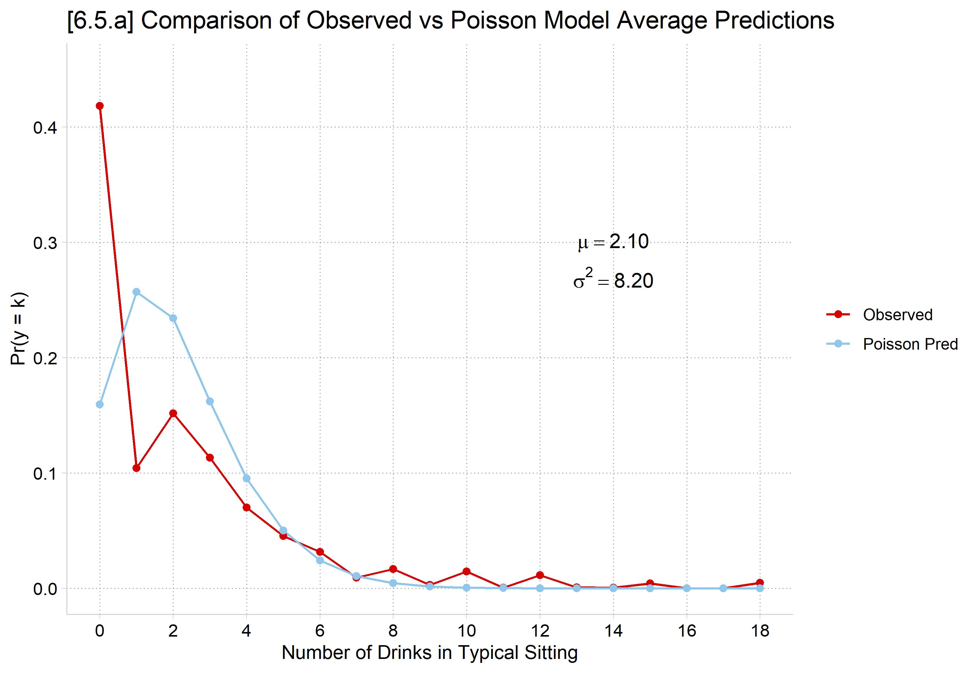
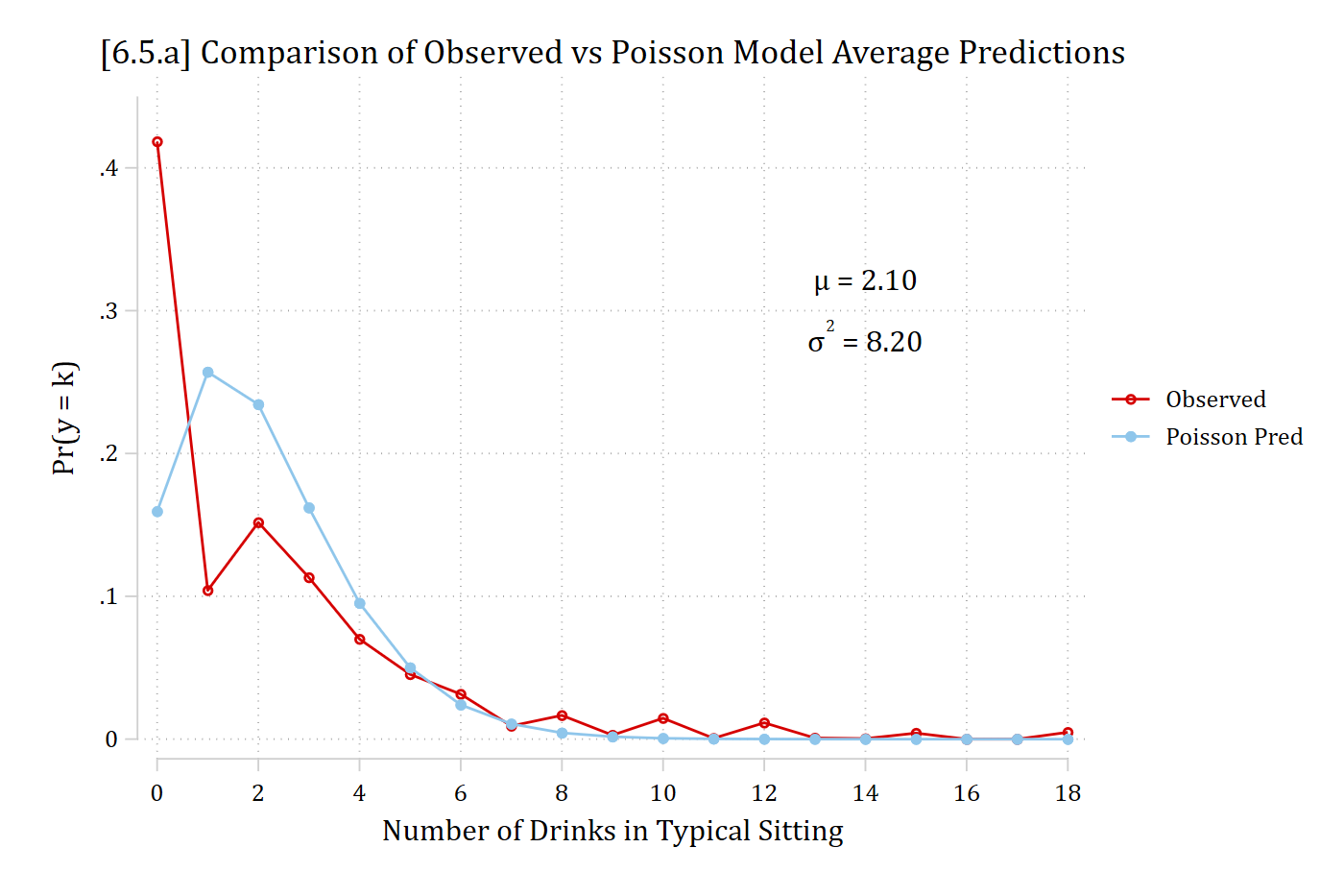
• Mean predicted probabilities summarizes model predictions

\[\overline{\Pr}(y = j) = \frac{1}{N}\sum_{i = 1}^{N}\Pr(y_{i} = j\,|\,\mathbf{x}_{i})\]

• Observed probability

\[\Pr_{observed}(y = j) = \frac{n_{y = j}}{N}\]

• If model is correct, we expect \(\overline{\Pr}(y = j) \approx \Pr_{observed}(y = j)\)

Stata

use "https://tdmize.github.io/data/data/cda_ah4", clear

(cda_ah4.dta | Add Health Wave 4 - | )

*6.5.a
qui poisson drinktime i.woman c.age i.college i.race c.income ///
    i.spouserole i.parrole, nolog
qui mgen, pr(0/18) meanpred stub(pmod) replace
twoway connected pmodobeq pmodpreq pmodval, ylab(0(.1).45) xlab(0(2)18) ///
    ytitle("Pr(y = k)") xtitle("Number of Drinks in Typical Sitting") ///
    title("[6.5.a] Comparison of Observed vs Poisson Model Average Predictions
") ///
    text(.3 14 "{&mu} = 2.10" " " "{&sigma}{sup:2} = 8.20") ///
    legend(order(1 "Observed" 2 "Poisson Pred"))

R

library(haven)           # import Stata data and labels
library(dplyr)           # data manipulation
library(tidyr)           # reshape data: pivot_longer()
library(ggplot2)         # graphs
library(cleanplots)      # graph scheme
cleanplots_defaults()

ah4 <- read_dta("https://tdmize.github.io/data/data/cda_ah4.dta")

# Keep model variables; drop any missing data
ah4 <- ah4[c("drinktime", "woman", "age", "college", "race", "income", "spouserole",
  "parrole")]
ah4 <- ah4[complete.cases(ah4), ]
ah4 <- ah4 |>
  mutate(across(c(woman, college, race, spouserole, parrole), as_factor))

pmod <- glm(drinktime ~ woman + age + college + race + income + spouserole + parrole,
  family = "poisson", data = ah4)

# 6.5.a - Observed proportions and average predicted probabilities of each count
meanpred <- data.frame(k = 0:18) |>
  mutate(Observed = sapply(k, function(j) mean(ah4$drinktime == j)),
    "Poisson Pred" = sapply(k, function(j) mean(dpois(j, fitted(pmod))))) |>
  pivot_longer(-k, names_to = "type", values_to = "pr")

ggplot(meanpred, aes(x = k, y = pr, color = type)) +
  geom_line() + geom_point() +
  annotate("text", x = 14, y = .3, label = 'mu == "2.10"', parse = TRUE) +
  annotate("text", x = 14, y = .27, label = 'sigma^2 == "8.20"', parse = TRUE) +
  scale_x_continuous(breaks = seq(0, 18, 2)) +
  scale_y_continuous(breaks = seq(0, .4, .1), limits = c(0, .45)) +
  labs(title = "[6.5.a] Comparison of Observed vs Poisson Model Average Predictions",
    x = "Number of Drinks in Typical Sitting", y = "Pr(y = k)", color = NULL)