6.4 Poisson Regression Example

Software considerations

• Convergence (of the maximum likelihood estimates) is usually fast and problems are rarely encountered
  • Also true for negative binomial model (covered next)
• Convergence can be trickier for zero-inflated count models (covered end of this section)
  • But, lack of convergence generally indicates that model is not a good fit for your data and solution is to use a regular count model

Example

• Add Health Wave IV
  • DV: Number of drinks consumed in a typical sitting
  • IVs: Gender, Age (24 – 33)
  • Controls: Education, race, income, marital status, parental status

Stata

use "https://tdmize.github.io/data/data/cda_ah4", clear

(cda_ah4.dta | Add Health Wave 4 - | )

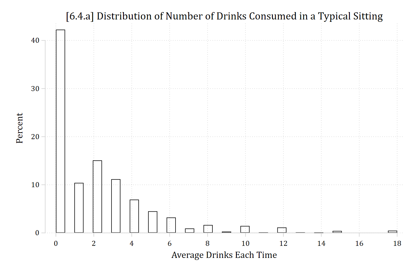
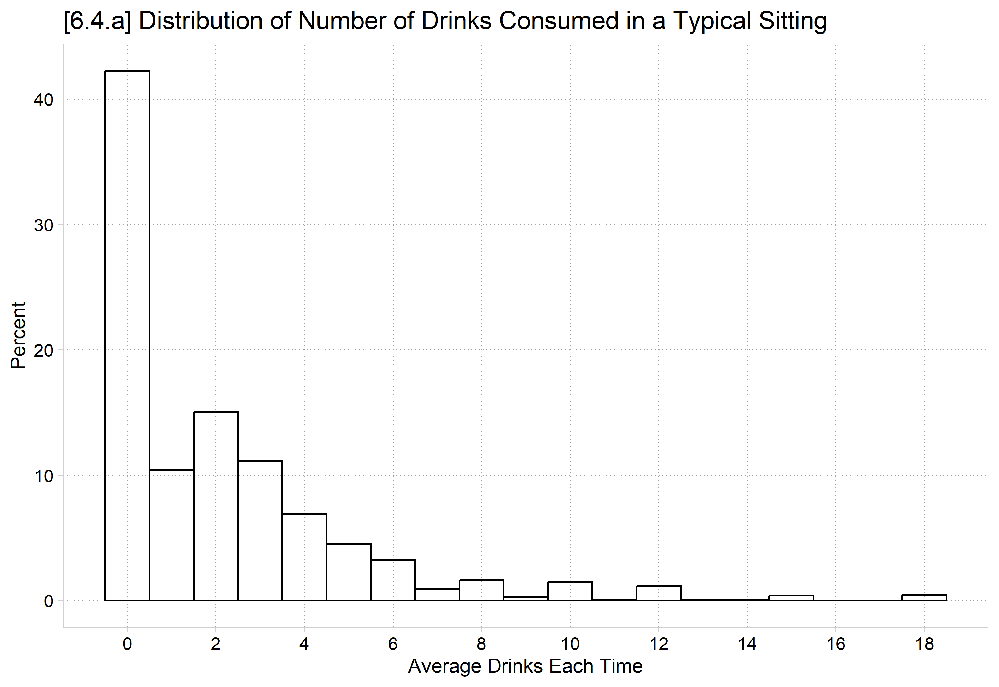
*6.4.a
hist drinktime, percent fcolor(none) xlab(0(2)18) ///
    title("[6.4.a] Distribution of Number of Drinks Consumed in a Typical Sitt
ing")

(bin=37, start=0, width=.48648649)

R

library(haven)           # import Stata data and labels
library(dplyr)           # data manipulation
library(ggplot2)         # graphs
library(modelsummary)    # regression tables
library(marginaleffects) # predictions and marginal effects
library(cleanplots)      # graph scheme
cleanplots_defaults()

ah4 <- read_dta("https://tdmize.github.io/data/data/cda_ah4.dta")

# 6.4.a
ggplot(ah4, aes(x = drinktime)) +
  geom_histogram(aes(y = after_stat(100 * count / sum(count))), binwidth = 1,
    fill = NA, color = "black") +
  scale_x_continuous(breaks = seq(0, 18, 2)) +
  labs(title = "[6.4.a] Distribution of Number of Drinks Consumed in a Typical Sitting",
    x = "Average Drinks Each Time", y = "Percent")

Stata

*6.4.b
poisson drinktime i.woman c.age i.college i.race c.income ///
    i.spouserole i.parrole

Iteration 0:  Log likelihood =  -11915.53  
Iteration 1:  Log likelihood = -11915.529  

Poisson regression                                     Number of obs =   4,983
                                                       LR chi2(9)    = 1610.51
                                                       Prob > chi2   =  0.0000
Log likelihood = -11915.529                            Pseudo R2     =  0.0633

-------------------------------------------------------------------------------
    drinktime | Coefficient  Std. err.      z    P>|z|     [95% conf. interval]
--------------+----------------------------------------------------------------
        woman |
       Woman  |     -0.496      0.021  -23.208   0.000       -0.538      -0.454
          age |     -0.051      0.005   -9.265   0.000       -0.061      -0.040
              |
      college |
College De..  |     -0.253      0.023  -10.869   0.000       -0.298      -0.207
              |
         race |
       Black  |     -0.367      0.026  -14.069   0.000       -0.418      -0.316
Native Ame..  |      0.286      0.093    3.085   0.002        0.104       0.467
       Asian  |     -0.132      0.058   -2.282   0.023       -0.246      -0.019
              |
       income |      0.003      0.000    7.931   0.000        0.002       0.004
              |
   spouserole |
     Married  |     -0.131      0.022   -6.065   0.000       -0.173      -0.089
              |
      parrole |
      Parent  |     -0.225      0.023   -9.697   0.000       -0.271      -0.180
        _cons |      2.642      0.154   17.153   0.000        2.340       2.944
-------------------------------------------------------------------------------

est store pmod
est table pmod, ///
    title("[6.4.b] Poisson regression for # of drinks in a sitting") ///
    b(%5.3f) star(.05 .01 .001)

[6.4.b] Poisson regression for # of drinks in a sitting

---------------------------
    Variable |    pmod     
-------------+-------------
       woman |
      Woman  |  -0.496***  
         age |  -0.051***  
             |
     college |
College D..  |  -0.253***  
             |
        race |
      Black  |  -0.367***  
Native Am..  |   0.286**   
      Asian  |  -0.132*    
             |
      income |   0.003***  
             |
  spouserole |
    Married  |  -0.131***  
             |
     parrole |
     Parent  |  -0.225***  
       _cons |   2.642***  
---------------------------
Legend: * p<.05; ** p<.01; *** p<.001

R

# Keep model variables; drop any missing data
ah4 <- ah4[c("drinktime", "woman", "age", "college", "race", "income", "spouserole",
  "parrole")]
ah4 <- ah4[complete.cases(ah4), ]

# Treat binary/nominal variables as factors
ah4 <- ah4 |>
  mutate(across(c(woman, college, race, spouserole, parrole), as_factor))

# 6.4.b
pmod <- glm(drinktime ~ woman + age + college + race + income + spouserole + parrole,
  family = "poisson", data = ah4)

modelsummary(pmod, stars = c("*" = .05, "**" = .01, "***" = .001),
  title = "[6.4.b] Poisson regression for # of drinks in a sitting")

[6.4.b] Poisson regression for # of drinks in a sitting

	(1)
* p < 0.05, ** p < 0.01, *** p < 0.001
(Intercept)	2.642***
	(0.154)
womanWoman	-0.496***
	(0.021)
age	-0.051***
	(0.005)
collegeCollege Degree	-0.253***
	(0.023)
raceBlack	-0.367***
	(0.026)
raceNative American	0.286**
	(0.093)
raceAsian	-0.132*
	(0.058)
income	0.003***
	(0.000)
spouseroleMarried	-0.131***
	(0.022)
parroleParent	-0.225***
	(0.023)
Num.Obs.	4983
AIC	23851.1
BIC	23916.2
Log.Lik.	-11915.529
F	173.906
RMSE	2.75

In Stata, use the poisson command

In R, use glm and specify family = “poisson”

Poisson regression coefficients are in the metric of the log rate—which is not very useful

We usually exponentiate the coefficients and interpret in terms of the factor change on the rate (see below)

Factor change in the rate E(y | x)

• To go from log rates to rates metric, we exponentiate the coefficients
  • This makes the coefficients multiplicative effects
• The effect of a change in x_k does not depend on values of the x’s

Factor change interpretation: For a unit change in x_k the expected count (rate) changes by a factor of exp(β_k), holding other variables constant

Interpreting factor changes in rate

Stata

*6.4.c - Exponentiated coefs with irr option
qui poisson drinktime i.woman c.age i.college i.race c.income ///
    i.spouserole i.parrole, irr
est table pmod, ///
    title("[6.4.c] Poisson regression for # of drinks in a sitting (exponentia
ted coefficients = IRRs)") ///
    b(%5.3f) star(.05 .01 .001) eform

[6.4.c] Poisson regression for # of drinks in a sitting (exponentiated
coefficients = IRRs)

---------------------------
    Variable |    pmod     
-------------+-------------
       woman |
      Woman  |   0.609***  
         age |   0.951***  
             |
     college |
College D..  |   0.777***  
             |
        race |
      Black  |   0.693***  
Native Am..  |   1.330**   
      Asian  |   0.876*    
             |
      income |   1.003***  
             |
  spouserole |
    Married  |   0.877***  
             |
     parrole |
     Parent  |   0.798***  
       _cons |  14.040***  
---------------------------
Legend: * p<.05; ** p<.01; *** p<.001

R

# 6.4.c - Exponentiated coefficients
exp(coef(pmod))

          (Intercept)            womanWoman                   age collegeCollege Degree 
           14.0395911             0.6089678             0.9506264             0.7766083 
            raceBlack   raceNative American             raceAsian                income 
            0.6929874             1.3304467             0.8761973             1.0028888 
    spouseroleMarried         parroleParent 
            0.8772996             0.7981304 

Exponentiated coefficients are referred to as “incident rate ratios” in Poisson

• Women’s rates of drinking are lower than men’s by a factor of about 0.61
• Each additional year of age is associated with a 0.95 times decrease in the number of drinks consumed in a sitting
• Black and Asian respondents drink fewer drinks in a sitting than do White respondents (e^b = 0.69; e^b = 0.88); in contrast, Native American respondents drink 1.33 times more drinks in a sitting than White respondents
• An additional $1000 of income is associated with consuming 1.003 times more drinks in a sitting

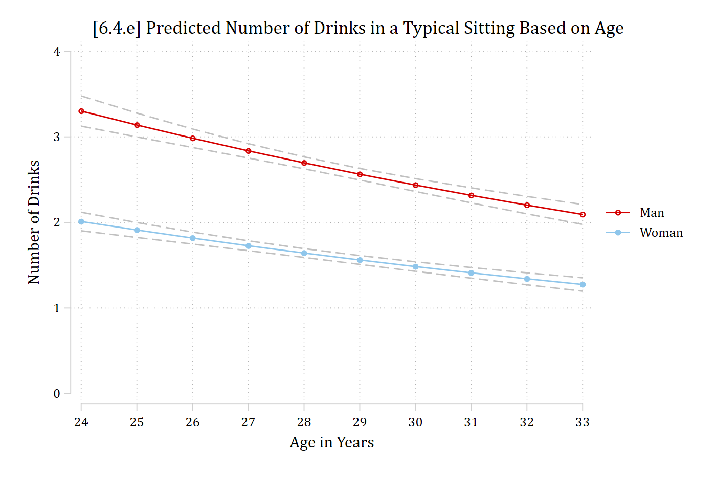
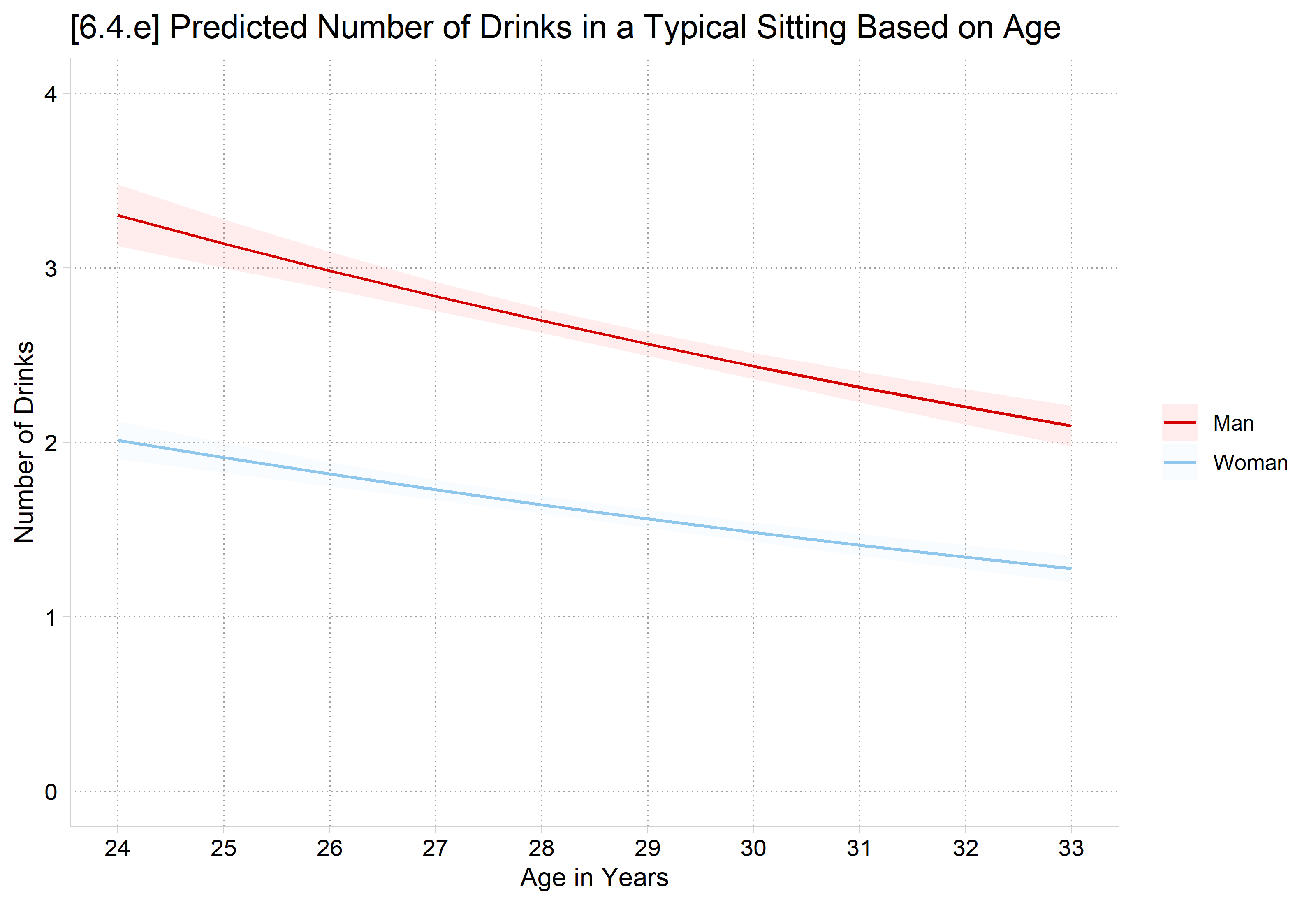
Plots of the predicted rate

• The predicted rate is the default quantity with margins in Stata and with plot_predictions in R
  • Easy to calculate

\[E(y) = \widehat{\mu} = \exp(\mathbf{x}\boldsymbol{\beta})\]

Stata

*6.4.e
qui margins, at(age=(24(1)33) woman=(0 1))
marginsplot, recastci(rline) ciopts(lpat(dash) col(gs12)) ylab(0(1)4) ///
    ytitle("Number of Drinks") xtitle("Age in Years") ///
    title("[6.4.e] Predicted Number of Drinks in a Typical Sitting Based on Ag
e", size(medium))

Variables that uniquely identify margins: age woman

R

R’s plot_predictions default would hold controls at modal person. To get average predictions, need the newdata statement with a “counterfactual” grid_type.

# 6.4.e
plot_predictions(pmod, by = c("age", "woman"),
  newdata = datagrid(age = 24:33, woman = unique, grid_type = "counterfactual")) +
  scale_x_continuous(breaks = 24:33) +
  scale_y_continuous(breaks = 0:4, limits = c(0, 4)) +
  labs(title = "[6.4.e] Predicted Number of Drinks in a Typical Sitting Based on Age",
    x = "Age in Years", y = "Number of Drinks", color = NULL, fill = NULL)

Stata

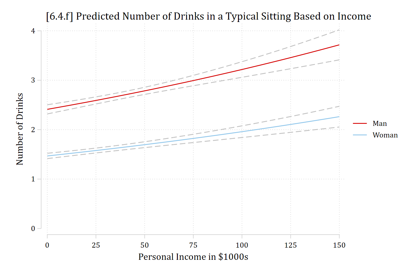
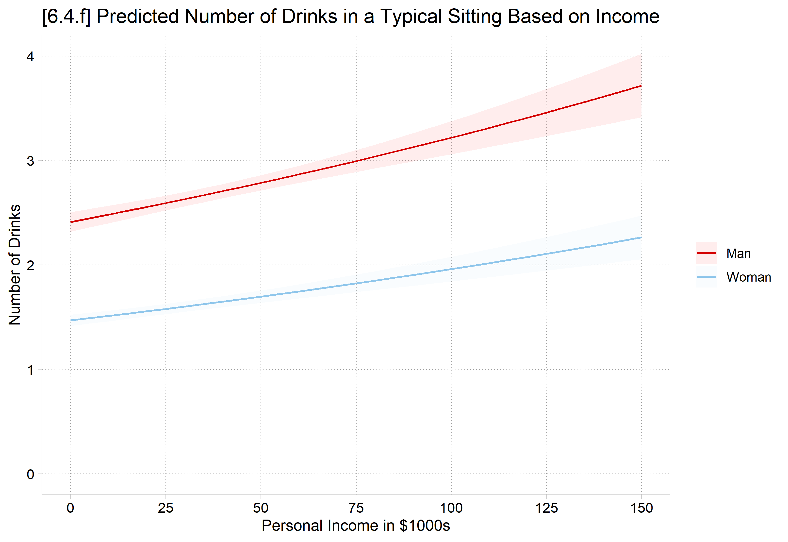
*6.4.f
qui margins, at(income=(0(5)150) woman=(0 1))
marginsplot, recastci(rline) ciopts(lpat(dash) col(gs12)) ylab(0(1)4) xlab(0(2
5)150) ///
    plotopts(msym(i)) ///
    ytitle("Number of Drinks") xtitle("Personal Income in $1000s") ///
    title("[6.4.f] Predicted Number of Drinks in a Typical Sitting Based on In
come", size(medium))

Variables that uniquely identify margins: income woman

R

# 6.4.f
plot_predictions(pmod, by = c("income", "woman"),
  newdata = datagrid(income = seq(0, 150, 5), woman = unique, grid_type = "counterfactual")) +
  scale_x_continuous(breaks = seq(0, 150, 25)) +
  scale_y_continuous(breaks = 0:4) +
  coord_cartesian(ylim = c(0, 4)) +
  labs(title = "[6.4.f] Predicted Number of Drinks in a Typical Sitting Based on Income",
    x = "Personal Income in $1000s", y = "Number of Drinks", color = NULL, fill = NULL)

Marginal effects on rates are not constant

Stata

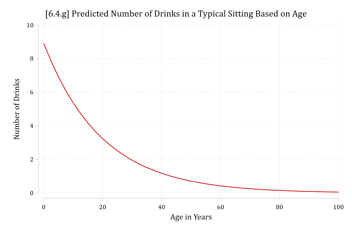
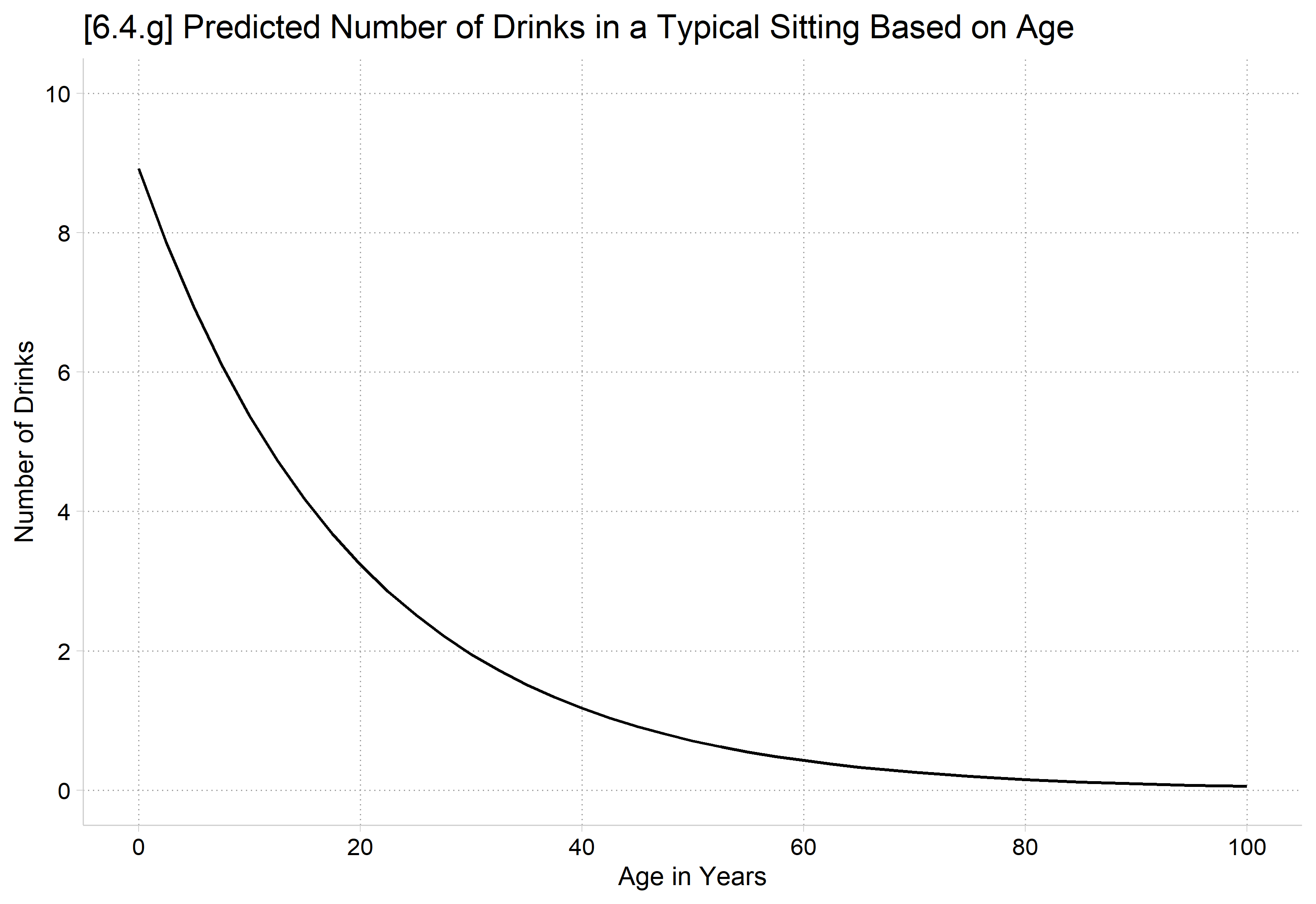
*Show nonlinearities (predictions across a broader range)
*6.4.g
qui margins, at(age=(0(2.5)100))
marginsplot, noci xlab(0(20)100) ylab(0(2)10) plotopts(msym(i)) ///
    ytitle("Number of Drinks") xtitle("Age in Years") ///
    title("[6.4.g] Predicted Number of Drinks in a Typical Sitting Based on Ag
e", size(medium))

Variables that uniquely identify margins: age

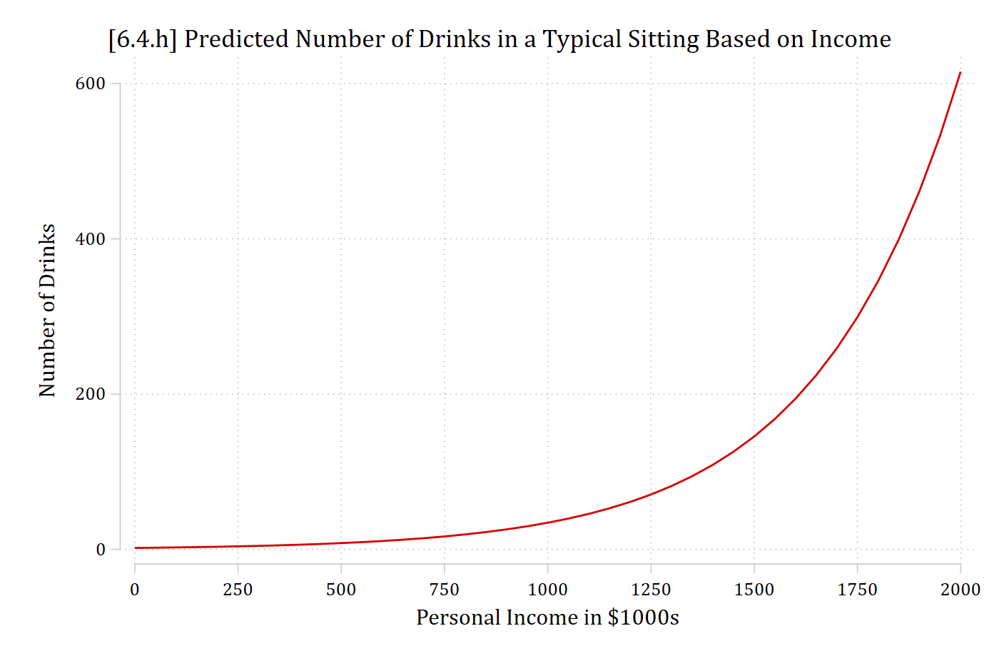
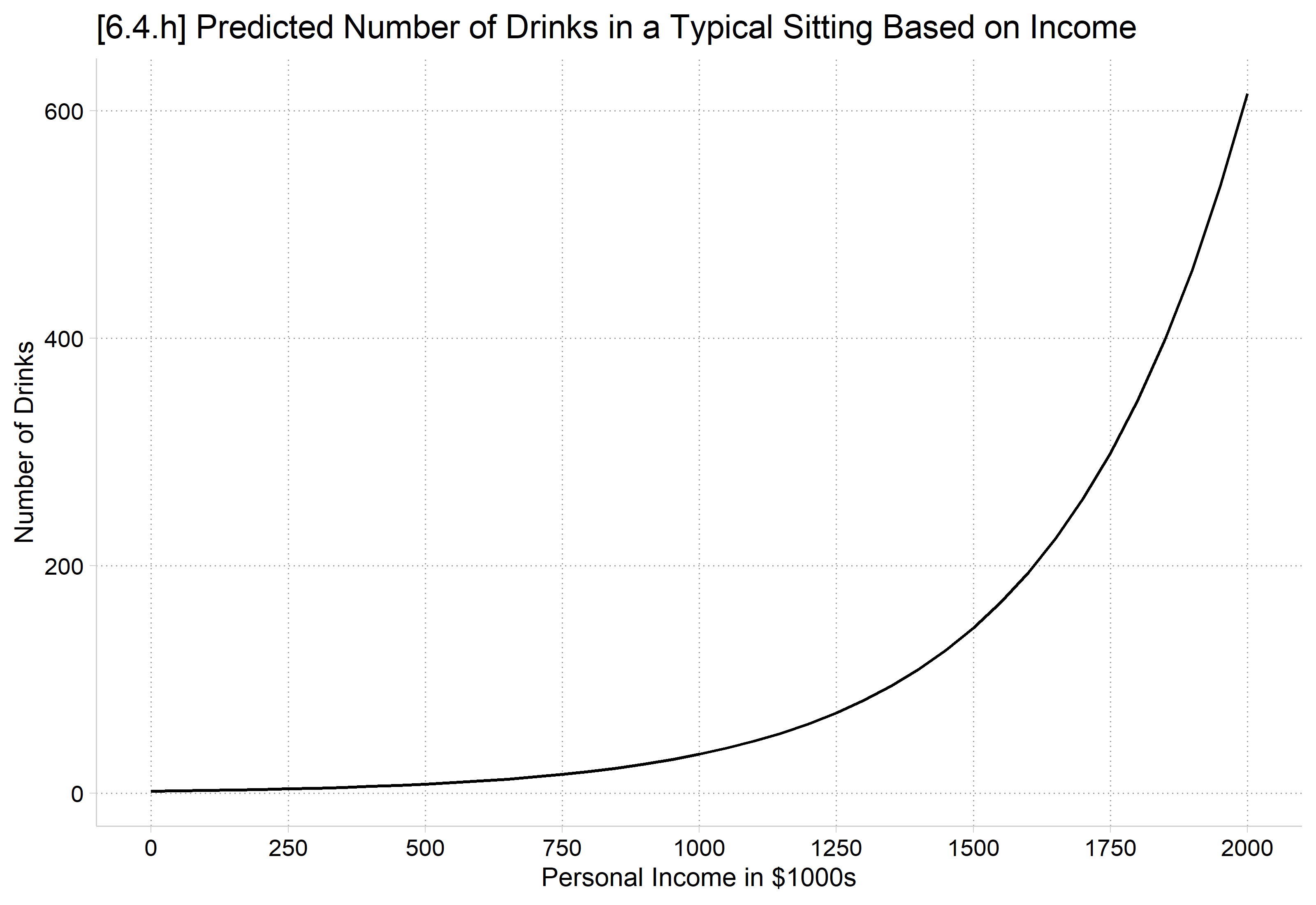
*6.4.h
qui margins, at(income=(0(50)2000))
marginsplot, noci ylab() xlab(0(250)2000) ///
    plotopts(msym(i)) ///
    ytitle("Number of Drinks") xtitle("Personal Income in $1000s") ///
    title("[6.4.h] Predicted Number of Drinks in a Typical Sitting Based on In
come", size(medium))

Variables that uniquely identify margins: income

R

# Show nonlinearities (predictions across a broader range)
# 6.4.g
plot_predictions(pmod, by = "age",
  newdata = datagrid(age = seq(0, 100, 2.5), grid_type = "counterfactual"), vcov = FALSE) +
  scale_x_continuous(breaks = seq(0, 100, 20)) +
  scale_y_continuous(breaks = seq(0, 10, 2), limits = c(0, 10)) +
  labs(title = "[6.4.g] Predicted Number of Drinks in a Typical Sitting Based on Age",
    x = "Age in Years", y = "Number of Drinks")

# 6.4.h
plot_predictions(pmod, by = "income",
  newdata = datagrid(income = seq(0, 2000, 50), grid_type = "counterfactual"), vcov = FALSE) +
  scale_x_continuous(breaks = seq(0, 2000, 250)) +
  labs(title = "[6.4.h] Predicted Number of Drinks in a Typical Sitting Based on Income",
    x = "Personal Income in $1000s", y = "Number of Drinks")

Marginal effect on the rate

• The factor change (e^b) is constant; it does not differ across values of the IVs
• The marginal effect depends on the values of the IVs
  • Considerations about what starting and ending values to use; whether to hold control variables at the mean (MEM) or to average over observed values (AMEs) are identical in count models to other nonlinear models

\[ME = \eta(x_{k} = end,\, \mathbf{x}_{-k} = \mathbf{x}^{*}) - \eta(x_{k} = start,\, \mathbf{x}_{-k} = \mathbf{x}^{*})\]

• There are multiple potential predictions of interest with count models
  • Can define \(\eta\) as the rate (AKA expected count; AKA # of expected “events”)
  • Can define \(\eta\) as the Pr(y = j)
  • Can define \(\eta\) as the probability of a range of outcomes, e.g., Pr(y = 4,5,6,7, or 8)
• For marginal effects on the rate/count:

Interpretation: The difference in the expected count for a change in x_k of δ, holding other independent variables constant

Stata

mecompare woman, model(pmod)

Predicting: Predicted number of events
Marginal effects (N_pmod=4983)

                                 |  ME #   Estimate         SE      P>|z|
---------------------------------+---------------------------------------
woman                            |                                       
                 Woman - Man     |                                       
                            pmod |     1     -1.038      0.045      0.000

R

avg_comparisons(pmod, variables = "woman")

 Estimate Std. Error     z Pr(>|z|)     S 2.5 % 97.5 %
    -1.04     0.0447 -23.2   <0.001 393.8 -1.13  -0.95

Term: woman
Type: response
Comparison: Woman - Man

On average, women consume about one fewer drink in a typical sitting than do men (ME = -1.038; p < 0.001).

Interpretation tip: Count DVs tend to have a natural metric; using it in your interpretations instead of “rate” or “expected count” is recommended. Here, “number of drinks”.

Stata

With mecompare, can customize start() place of change, and the amount(#) of change. uncenter the change if you want an ME between those two exact #s.

mecompare age, model(pmod) start(age=25) amount(5) uncenter

Predicting: Predicted number of events
Marginal effects (N_pmod=4983)

                                 |  ME #   Estimate         SE      P>|z|
---------------------------------+---------------------------------------
age + 5 (uncentered)             |                                       
                            pmod |     1     -0.562      0.064      0.000

R

avg_comparisons(pmod, variables = list(age = c(25, 30)))

 Estimate Std. Error     z Pr(>|z|)    S  2.5 % 97.5 %
   -0.562     0.0636 -8.84   <0.001 59.9 -0.687 -0.438

Term: age
Type: response
Comparison: 30 - 25

Aging from 25 to 30 is associated with consuming about ½ a drink less per sitting (ME = -0.562; p < 0.001).

Probabilities of specific counts

• For a given rate, the probability of count j for observation i is:

\[\Pr(y_{i} = j\,|\,\mathbf{x}_{i}) = \frac{e^{-\widehat{\mu}_{i}}\,\widehat{\mu}_{i}^{\,j}}{j!}\]

• Sometimes the probability of specific count is of interest
  • Pr(y = 0) is commonly of interest
  • Depending on research question, probabilities at other values and/or cumulative probabilities may be of interest
    • E.g., To determine who is at risk, examine what the probability is that someone consumes ≥ 4 drinks in a typical sitting: Pr(y ≥ 4)
• Probabilities are also used to assess the adequacy of the model

Plotting probabilities of specific counts

Stata

• In Stata, can request the probability of a specific count # on margins, with option predict(pr(#))
  • And a range with predict(pr(#,#))

*6.4.i - Pr(y=0)
est restore pmod

(results pmod are active now)

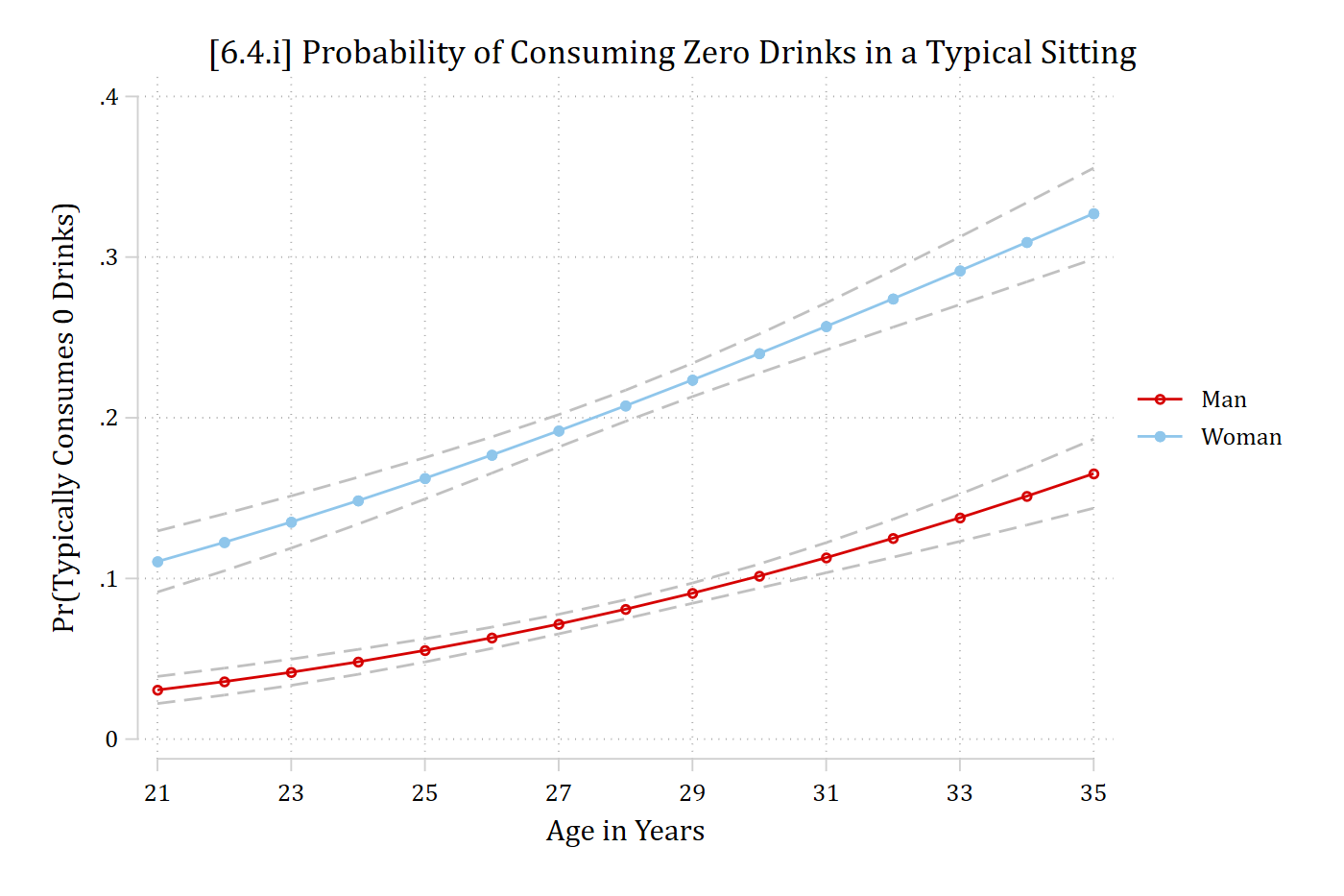
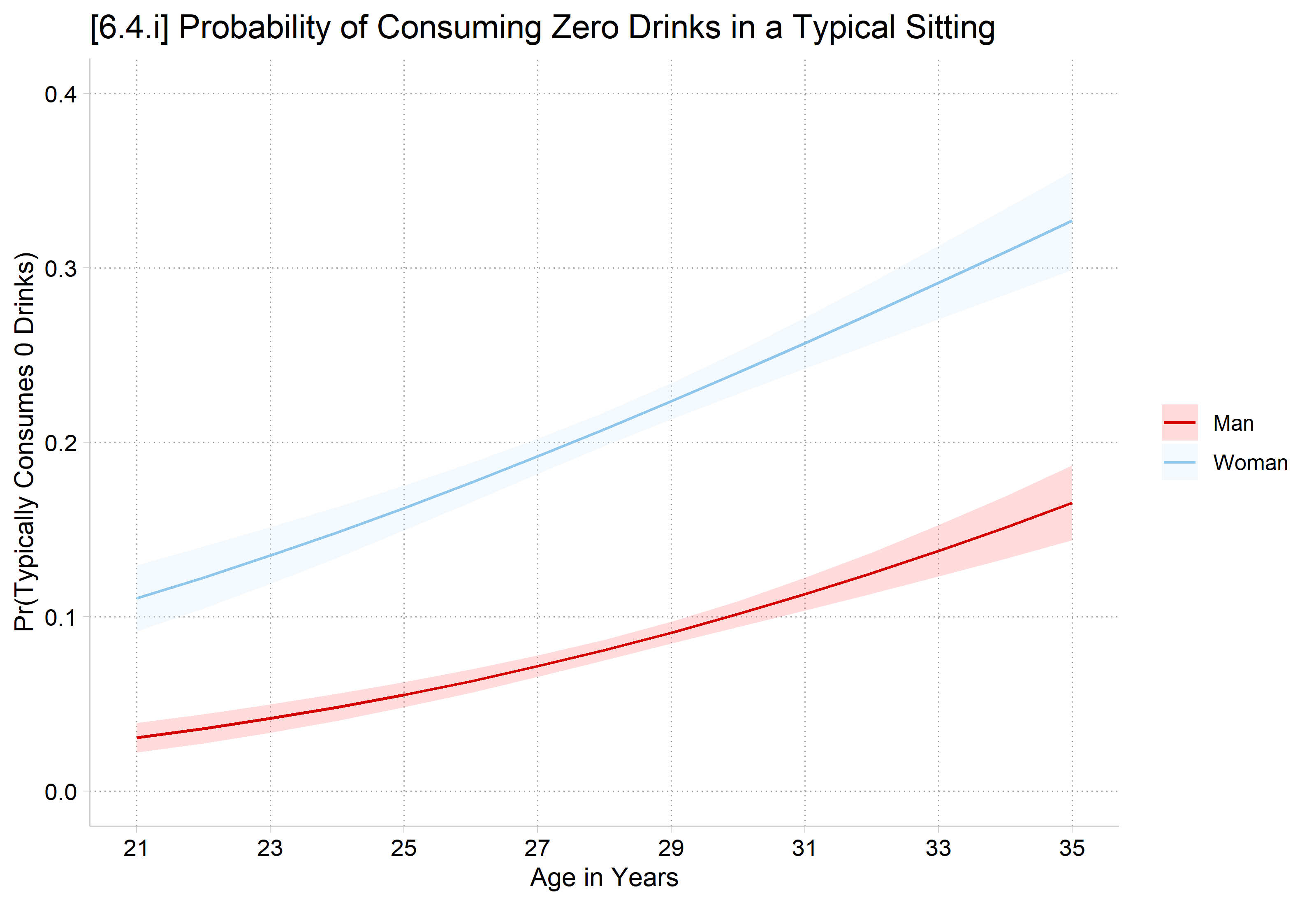
qui margins, at(age=(21(1)35) woman=(0 1)) predict(pr(0))
marginsplot, recastci(rline) ciopts(lpat(dash) col(gs12)) ylab(0(.1).4) xlab(2
1(2)35) ///
    ytitle("Pr(Typically Consumes 0 Drinks)") xtitle("Age in Years") ///
    title("[6.4.i] Probability of Consuming Zero Drinks in a Typical Sitting",
 size(medium))

Variables that uniquely identify margins: age woman

R

• In R, plot_predictions only predicts the expected count
  • Instead, use predictions() first and convert each person’s predicted count to the probability of a specific count with dpois(#, x) inside the hypothesis option
    • Take the mean() to average within each age and gender combination
  • Use ggplot to make the graph using the stored predictions

# 6.4.i - Pr(y=0)
pr0 <- predictions(pmod, type = "response",
  newdata = datagrid(age = 21:35, woman = unique, grid_type = "counterfactual"),
  hypothesis = ~ I(mean(dpois(0, x))) | age + woman)

ggplot(pr0, aes(age, estimate, ymin = conf.low, ymax = conf.high, color = woman, fill = woman)) +
  geom_ribbon(alpha = .2, color = NA) + geom_line() +
  scale_x_continuous(breaks = seq(21, 35, 2)) +
  scale_y_continuous(breaks = seq(0, .4, .1), limits = c(0, .4)) +
  labs(title = "[6.4.i] Probability of Consuming Zero Drinks in a Typical Sitting",
    x = "Age in Years", y = "Pr(Typically Consumes 0 Drinks)", color = NULL, fill = NULL)

Marginal effects on probabilities of specific counts

• Define \(\eta\) as the probability of a specific count # (or range)

\[\eta = \Pr(y = j\,|\,\mathbf{x}_{i}) = \frac{e^{-\widehat{\mu}_{i}}\,\widehat{\mu}_{i}^{\,j}}{j!}\]

• Marginal effect is difference in probability of specific count, conditional on two values of the focal IV of interest

\[ME = \eta(x_{k} = end,\, \mathbf{x}_{-k} = \mathbf{x}^{*}) - \eta(x_{k} = start,\, \mathbf{x}_{-k} = \mathbf{x}^{*})\]

Interpretation: The difference in the probability of a count of # for a change in x_k of δ, holding other independent variables constant

• And for a range of counts

Interpretation: The difference in the probability of a count between # and # for a change in x_k of δ, holding other independent variables constant

Stata

*NOTE: Pass customized predict() functions
mecompare age, model(pmod) amount(trimrange) predict(pr(0))

Predicting: Pr(drinktime=0)
Marginal effects (N_pmod=4983)

                                 |  ME #   Estimate         SE      P>|z|
---------------------------------+---------------------------------------
age(5-95%)                       |                                       
                            pmod |     1      0.065      0.007      0.000

R

avg_comparisons(pmod, variables = list(age = c(26, 31)),
  comparison = function(hi, lo) dpois(0, hi) - dpois(0, lo))

 Estimate Std. Error    z Pr(>|z|)    S  2.5 % 97.5 %
   0.0654    0.00712 9.18   <0.001 64.4 0.0514 0.0793

Term: age
Type: response
Comparison: custom

Aging from the 5^th to 95^th percentile in the data (26 to 31), predicts a 6.5 percentage point increase in the probability of not drinking any alcoholic drinks.

Interpretation tip: As with a +SD effect, the first time you report a (trimmed) range ME, useful to remind readers what those values are in your data.

Stata

*6.4.j - Pr(y=3)
est restore pmod

(results pmod are active now)

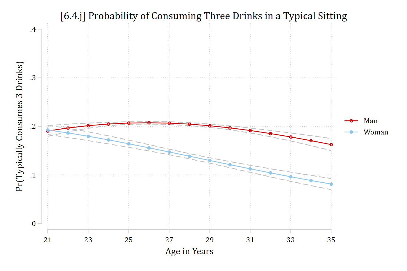
qui margins, at(age=(21(1)35) woman=(0 1)) predict(pr(3))
marginsplot, recastci(rline) ciopts(lpat(dash) col(gs12)) ylab(0(.1).4) xlab(2
1(2)35) ///
    ytitle("Pr(Typically Consumes 3 Drinks)") xtitle("Age in Years") ///
    title("[6.4.j] Probability of Consuming Three Drinks in a Typical Sitting"
, size(medium))

Variables that uniquely identify margins: age woman

R

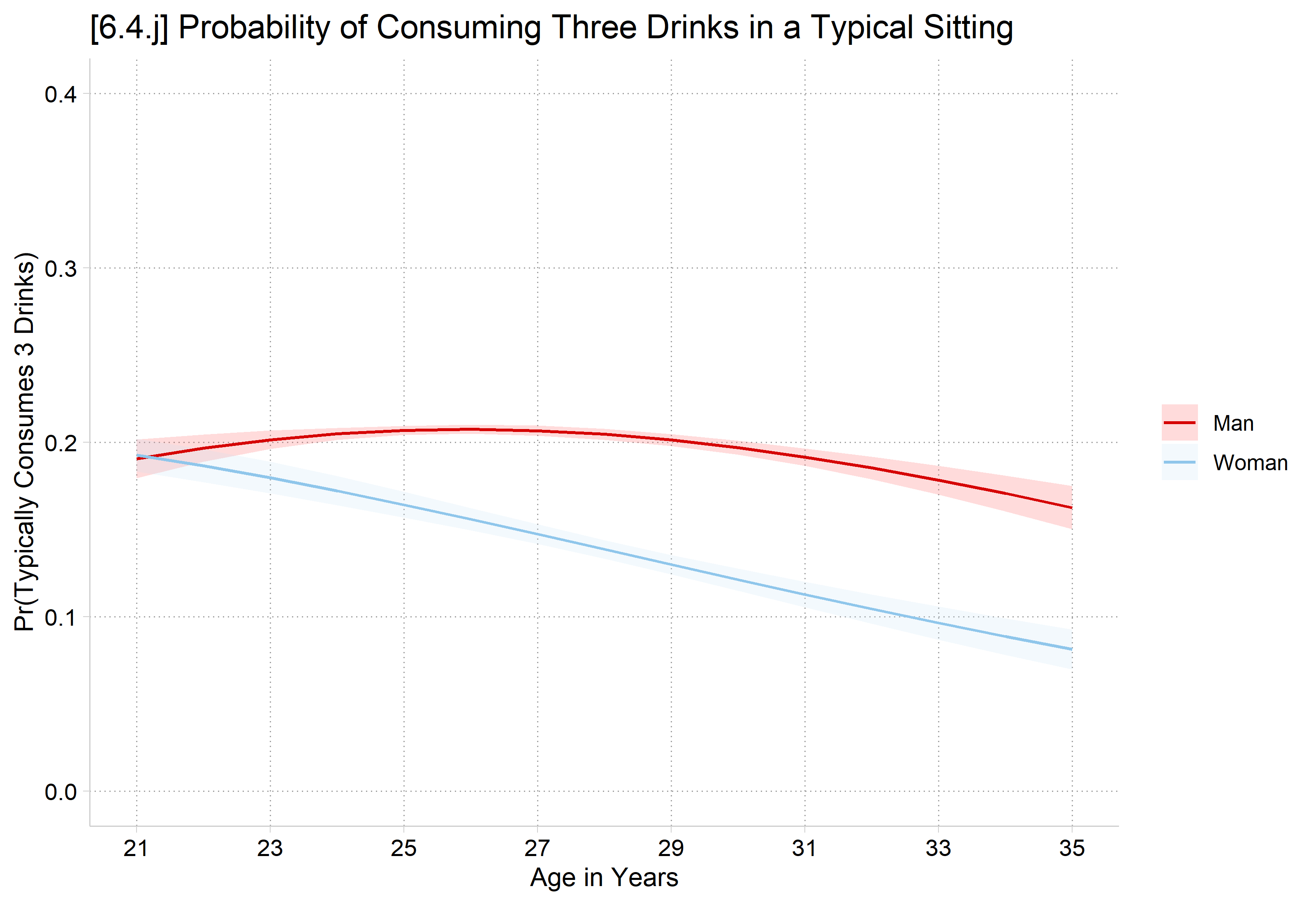
# 6.4.j - Pr(y=3)
pr3 <- predictions(pmod, type = "response",
  newdata = datagrid(age = 21:35, woman = unique, grid_type = "counterfactual"),
  hypothesis = ~ I(mean(dpois(3, x))) | age + woman)

ggplot(pr3, aes(age, estimate, ymin = conf.low, ymax = conf.high, color = woman, fill = woman)) +
  geom_ribbon(alpha = .2, color = NA) + geom_line() +
  scale_x_continuous(breaks = seq(21, 35, 2)) +
  scale_y_continuous(breaks = seq(0, .4, .1), limits = c(0, .4)) +
  labs(title = "[6.4.j] Probability of Consuming Three Drinks in a Typical Sitting",
    x = "Age in Years", y = "Pr(Typically Consumes 3 Drinks)", color = NULL, fill = NULL)

Stata

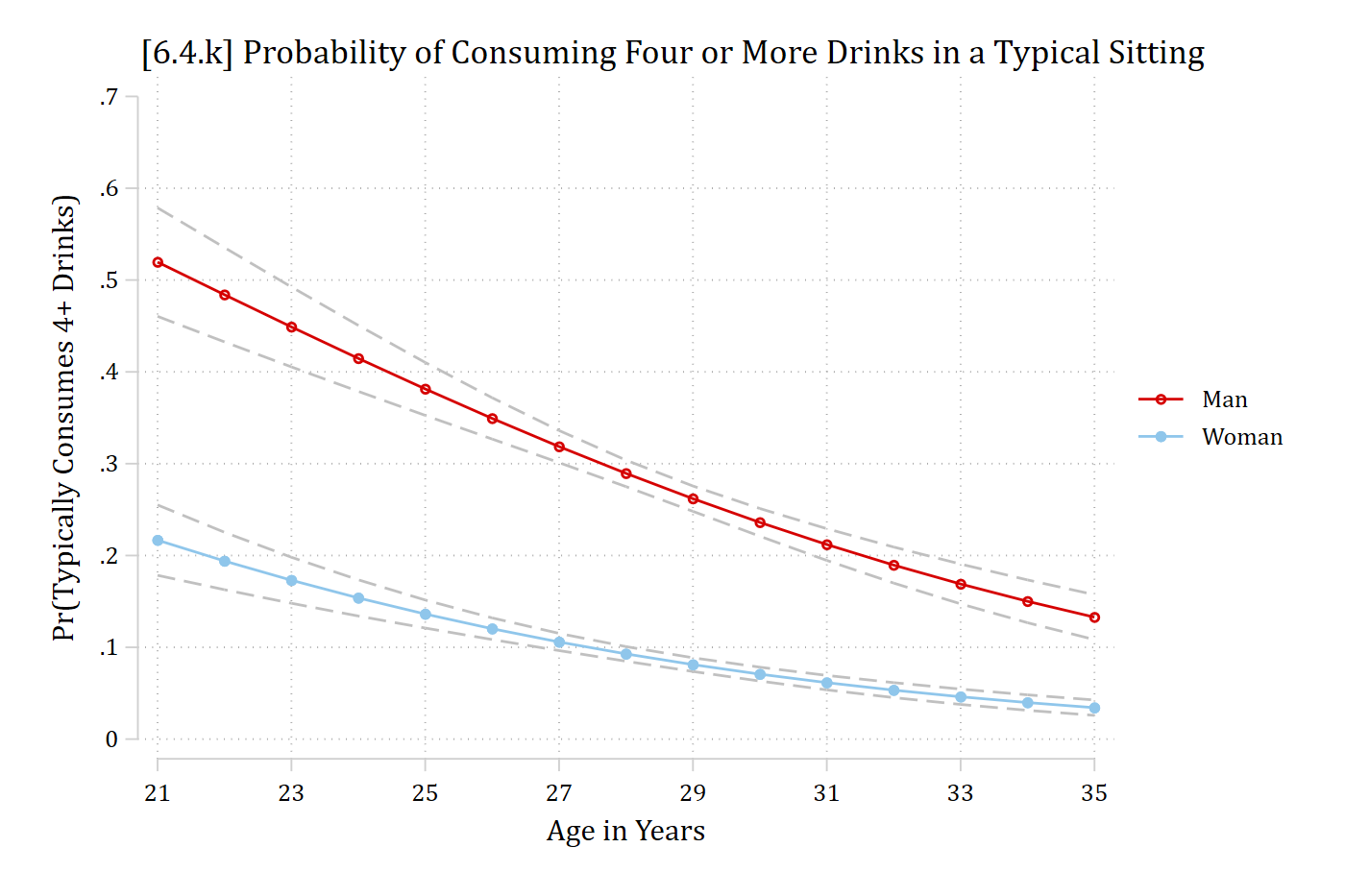
*6.4.k - Pr(y >= 4)
qui margins, at(age=(21(1)35) woman=(0 1)) predict(pr(4,18))
marginsplot, recastci(rline) ciopts(lpat(dash) col(gs12)) ylab(0(.1).7) xlab(2
1(2)35) ///
    ytitle("Pr(Typically Consumes 4+ Drinks)") xtitle("Age in Years") ///
    title("[6.4.k] Probability of Consuming Four or More Drinks in a Typical S
itting", size(medium))

Variables that uniquely identify margins: age woman

R

• In R, for a range of counts, use ppois(#, x), which gives the probability of # or fewer. Specify amount between end # and start # – 1. E.g. For Pr(y = 4–18)

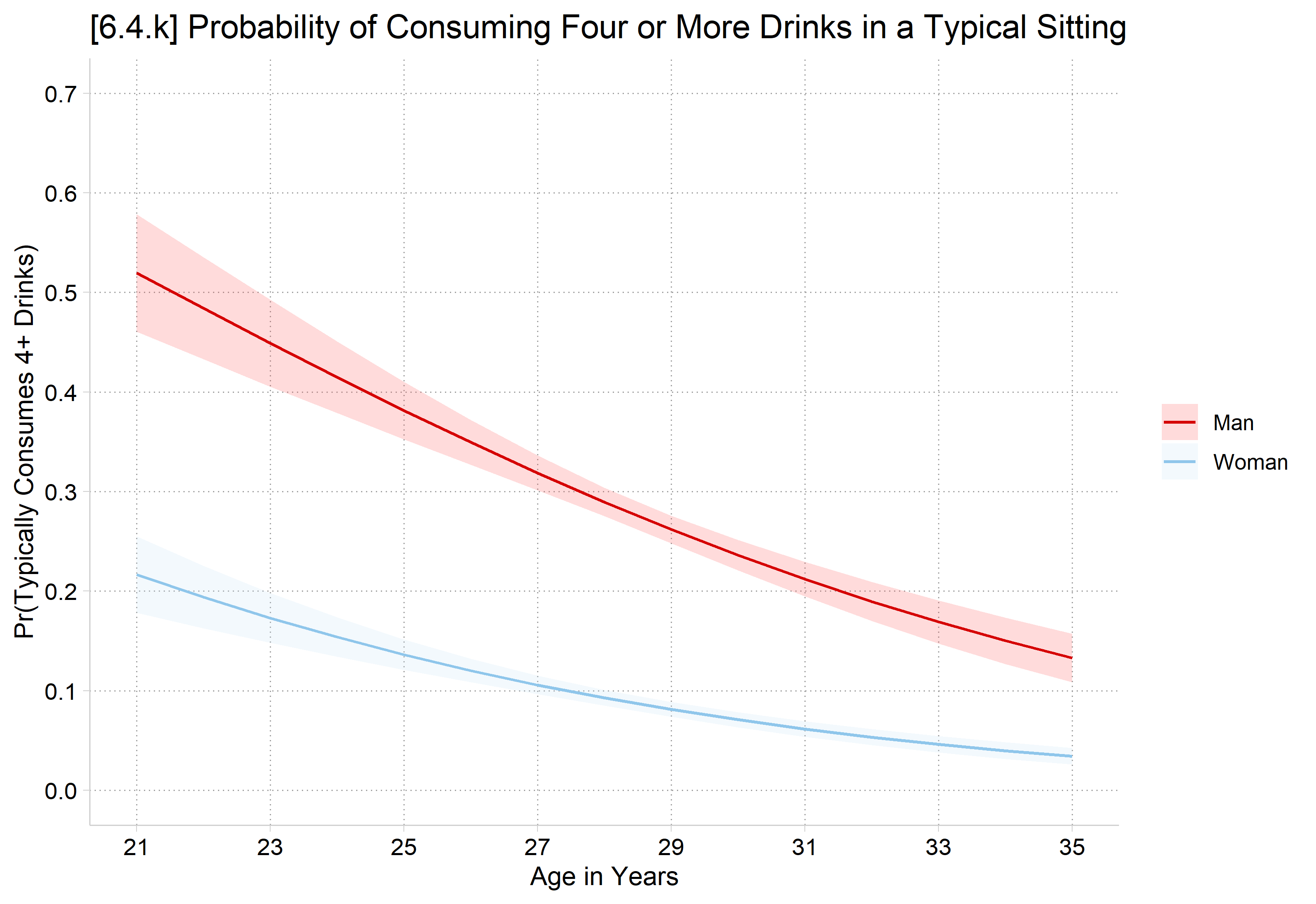
# 6.4.k - Pr(y >= 4)
pr4_18 <- predictions(pmod, type = "response",
  newdata = datagrid(age = 21:35, woman = unique, grid_type = "counterfactual"),
  hypothesis = ~ I(mean(ppois(18, x) - ppois(3, x))) | age + woman)

ggplot(pr4_18, aes(age, estimate, ymin = conf.low, ymax = conf.high, color = woman, fill = woman)) +
  geom_ribbon(alpha = .2, color = NA) + geom_line() +
  scale_x_continuous(breaks = seq(21, 35, 2)) +
  scale_y_continuous(breaks = seq(0, .7, .1), limits = c(0, .7)) +
  labs(title = "[6.4.k] Probability of Consuming Four or More Drinks in a Typical Sitting",
    x = "Age in Years", y = "Pr(Typically Consumes 4+ Drinks)", color = NULL, fill = NULL)

Marginal effects on probability of a range of counts

Stata

mecompare age, model(pmod) amount(sd) predict(pr(4,18))

Predicting: Pr(4<=drinktime<=18)
Marginal effects (N_pmod=4983)

                                 |  ME #   Estimate         SE      P>|z|
---------------------------------+---------------------------------------
age + SD (centered)              |                                       
                            pmod |     1     -0.035      0.004      0.000

R

# Center changes in continuous IVs on each observation's value (as mecompare does)
options(marginaleffects_contrast_direction = "center")

avg_comparisons(pmod, variables = list(age = sd(ah4$age)),
  comparison = function(hi, lo) (ppois(18, hi) - ppois(3, hi)) - (ppois(18, lo) - ppois(3, lo)))

 Estimate Std. Error    z Pr(>|z|)    S   2.5 %  97.5 %
   -0.035    0.00376 -9.3   <0.001 66.0 -0.0423 -0.0276

Term: age
Type: response
Comparison: +1.81236443621303

In this article, we define risk of alcohol misuse as reporting an average number of alcoholic drinks in a sitting as 4 or more. Using this definition, aging a standard deviation (about 2 years) predicts a 3.5 percentage point decrease in the probability of being at risk of alcohol misuse.