Excessive decoration/color should be avoided (but see my caveat below)
All aspects of the graph should aid in presenting the data
The “data ink” ratio should be as high as possible (Tufte 1983)
The basic idea behind this principle: all aspects of a graphic should serve the purpose of showing the data
Consider whether superfluous additional pieces/colors on your graphic can be removed
My less strict rule: all color should convey some information
The data-ink ratio: my caveat
“… ‘remove clutter and strive for clean and elegant designs’… is reasonable advice. But… ‘do everything you can to remove non-data ink’…will result in poor design choices.” (Wilke 2019 p.277-278)
I am much less of a fundamentalist about the maximize data ink rule
In the age of PDFs and online journals/reports/websites, it isn’t “wasteful” to include extra color or other data ink
Sometimes the color displays useful information (e.g., your brain registers amount better with a bar chart than a dot plot because the blocks of color carry visual information on quantity)
Color can help you quickly identify different parts of the graph (e.g., the blue line shows…)
Sometimes the color… looks nice
Having aesthetically pleasing graphics is important
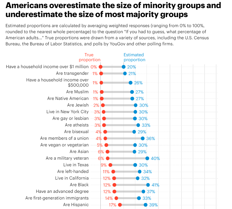
Dot plots
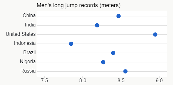
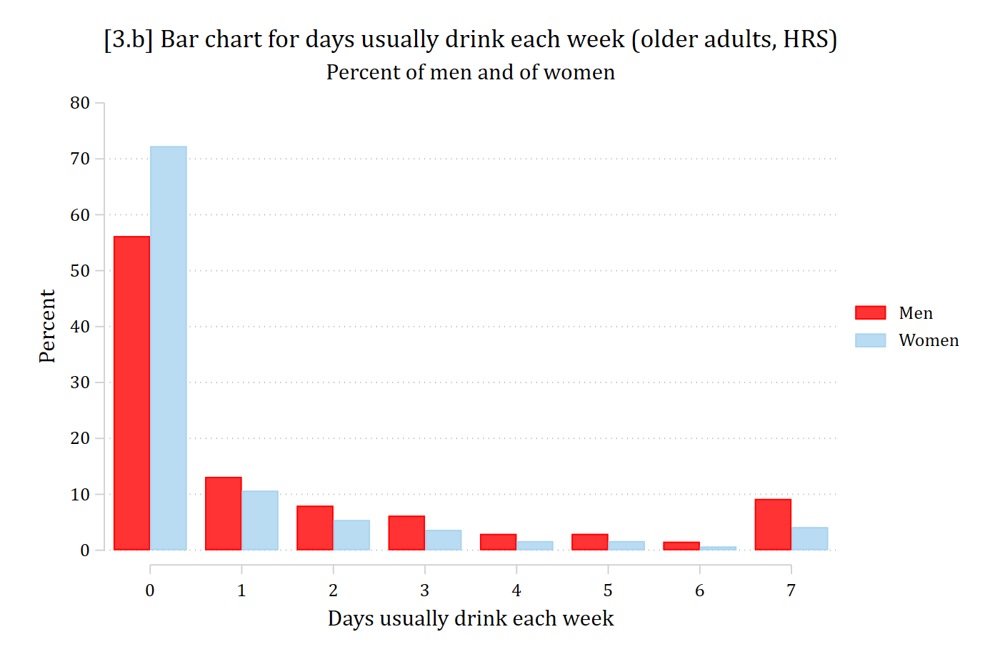
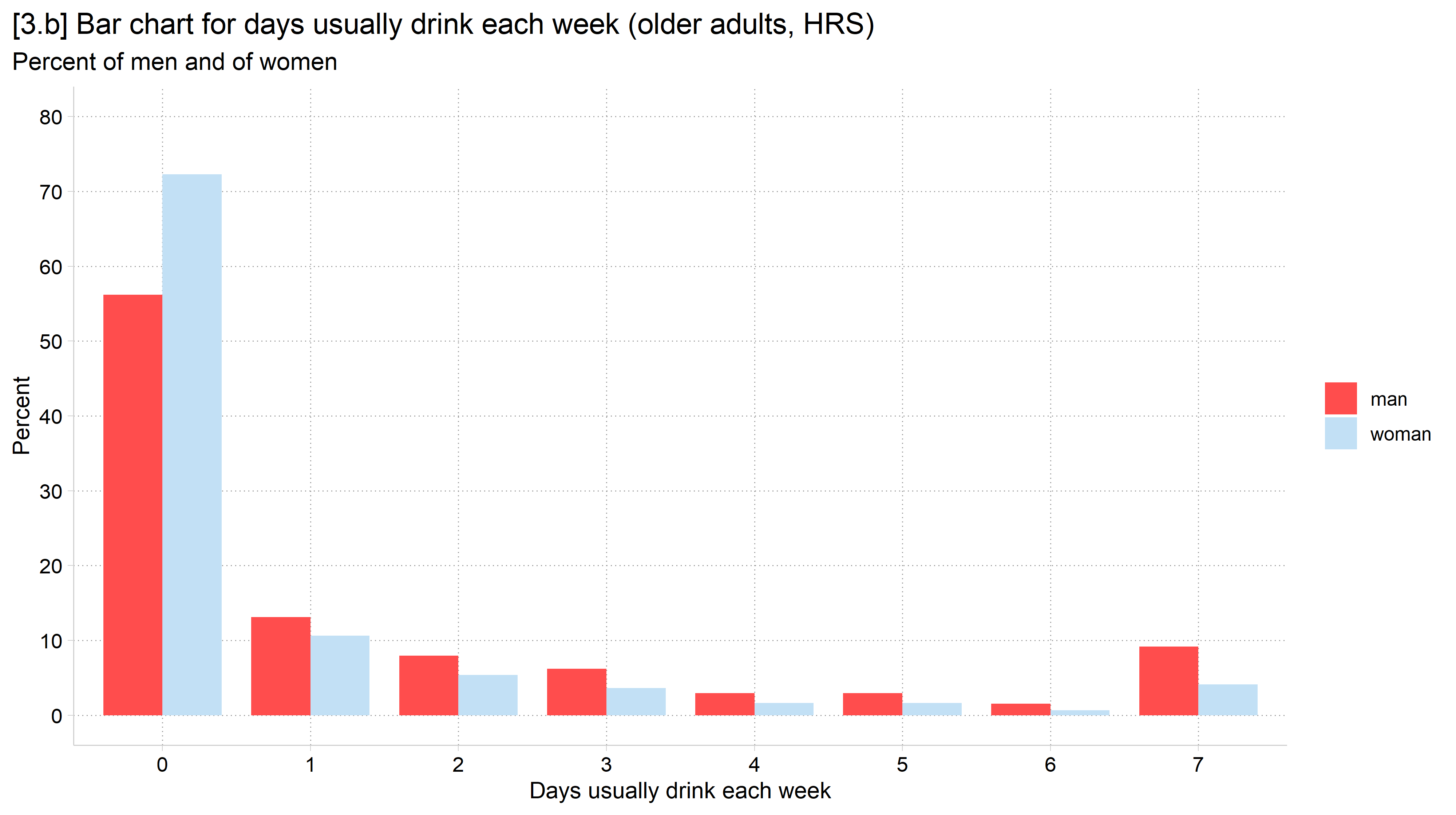
Dot plots can often be used interchangeably with bar charts
But, instead of a colored in bar, you simply place a dot at the value being plotted (would be the top of the bar)
Dot plots can similarly easily incorporate measures of uncertainty in the form of SEs or CIs
Dot plots were invented to take advantage of the knowledge gleaned from Cleveland and colleagues’ visual perception experiments and Tufte’s opinions about excess decoration
Advantages of dot plots
An advantage of dot plots is that they waste less data ink when compared to a bar chart (Tufte 1983)
This also keeps them from becoming crowded and unreadable
A purely utilitarian reason to use a dot plot is that people will give you a hard time for having a bar chart that does not start at zero—while no one seems to care if a dot plot starts at zero
There are good reasons for this concern as bar charts display information both as length and area—and the area can be misleading without a zero baseline
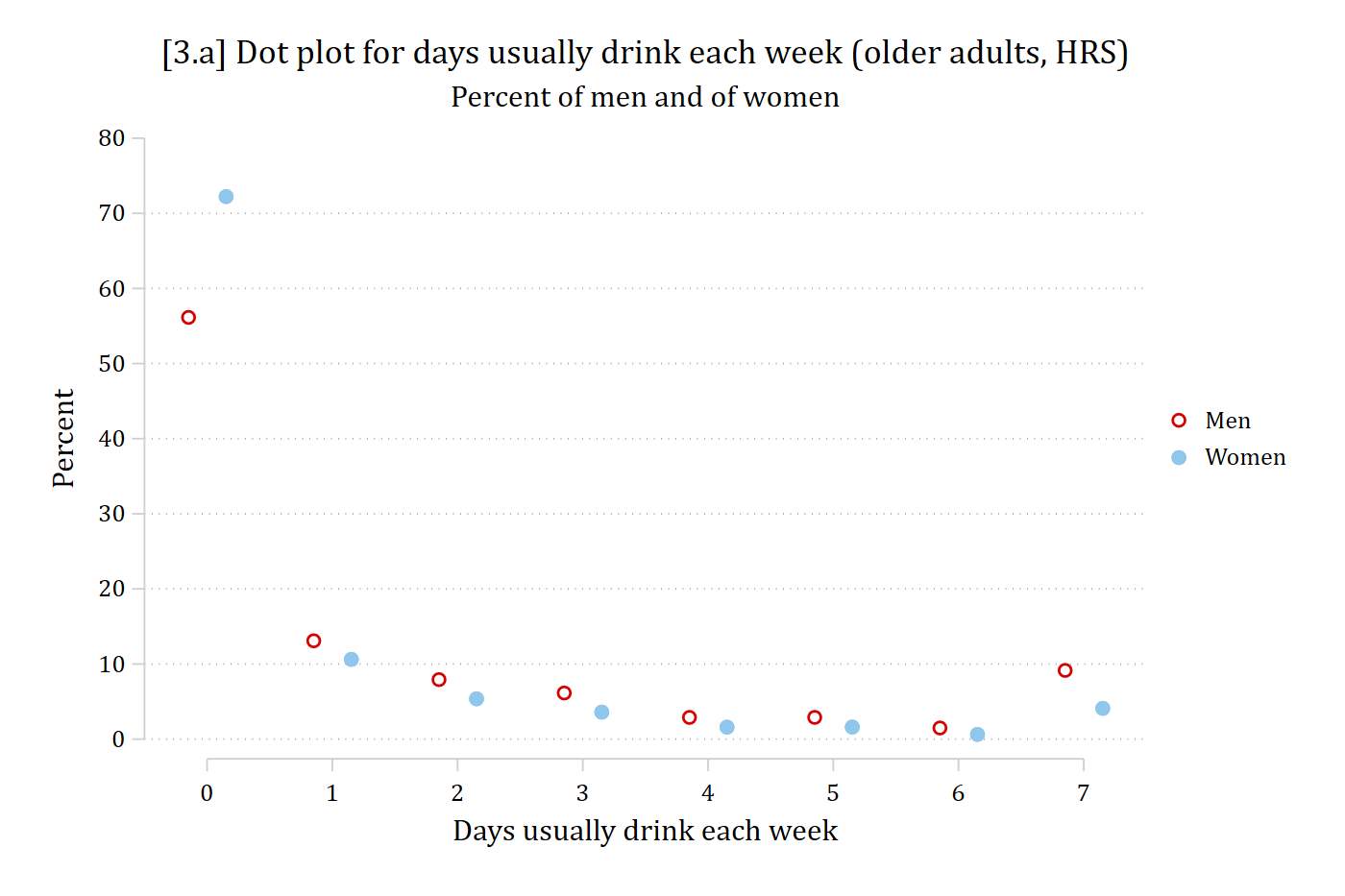
eststore drink_wom// 3.a - Dot plot for days drinking per week, by gendercoefplot (drink_men, label("Men") offset(-0.15)) /// (drink_wom, label("Women") offset(0.15)), /// vertical noci msize(*1.5) rescale(100) ylab(0(10)80) /// xlab(1 "0" 2 "1" 3 "2" 4 "3" 5 "4" 6 "5" 7 "6" 8 "7") ///ytitle("Percent") xtitle("Days usually drink each week") ///title("[3.a] Dot plot for days usually drink each week (older adults, HRS)") ///subtitle("Percent of men and of women")
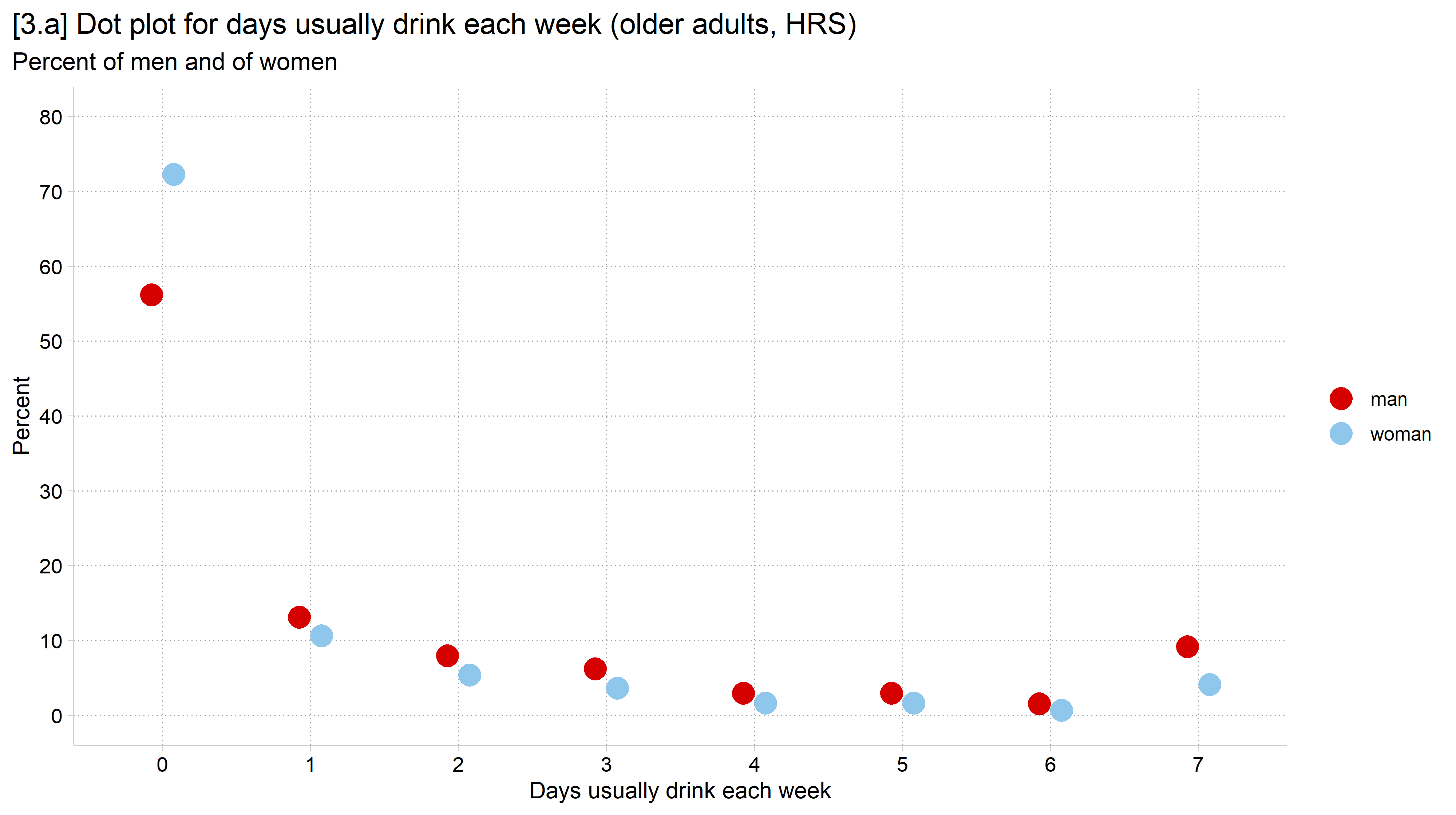
library(foreign) # load Stata datasetslibrary(ggplot2) # main graphics packagelibrary(dplyr) # data manipulation toolslibrary(cleanplots) # Mize's graphics scheme## Use cleanplots colors, markers, lines, and theme for all graphs ##cleanplots_defaults()theme_update(plot.title.position ="plot") # titles start at left edge of graph# Health and Retirement Study Datahrs <-read.dta("https://tdmize.github.io/data/data/hrs_si.dta")# Percent of men and of women in each category of days drinkingdrink_pct <- hrs %>%filter(!is.na(dayweekdrink)) %>%count(woman, dayweekdrink) %>%group_by(woman) %>%mutate(pct =100* n /sum(n))# 3.a - Dot plot for days drinking per week, by genderggplot(drink_pct, aes(x =factor(dayweekdrink), y = pct, color = woman)) +geom_point(size =4.5, position =position_dodge(width = .3)) +labs(x ="Days usually drink each week", y ="Percent", color ="",title ="[3.a] Dot plot for days usually drink each week (older adults, HRS)",subtitle ="Percent of men and of women") +scale_y_continuous(breaks =seq(0, 80, 10), limits =c(0, 80))
// 3.b - Same information as a bar chartcoefplot (drink_men, label("Men") offset(-0.2)) /// (drink_wom, label("Women") offset(0.2)), /// vertical noci rescale(100) ylab(0(10)80) ///recast(bar) barwidth(0.4) /// xlab(1 "0" 2 "1" 3 "2" 4 "3" 5 "4" 6 "5" 7 "6" 8 "7") ///ytitle("Percent") xtitle("Days usually drink each week") ///title("[3.b] Bar chart for days usually drink each week (older adults, HRS)") ///subtitle("Percent of men and of women")
# 3.b - Same information as a bar chartggplot(drink_pct, aes(x =factor(dayweekdrink), y = pct, fill = woman)) +geom_col(position =position_dodge(width = .8), width = .8) +labs(x ="Days usually drink each week", y ="Percent", fill ="",title ="[3.b] Bar chart for days usually drink each week (older adults, HRS)",subtitle ="Percent of men and of women") +scale_y_continuous(breaks =seq(0, 80, 10), limits =c(0, 80))