10. Don’t assume linearity

Scatterplots of two continuous variables

  • Scatterplots are among the most common and intuitive data visualization techniques
  • Plot each individual observation by placing one variable on the x-axis and another on the y-axis, and placing a dot where each observation falls
    • The dependent variable (DV) or outcome is the y-variable
    • The independent variable (IV) or cause is the x-variable

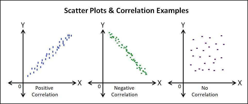
Three example scatterplots showing a positive correlation, a negative correlation, and no correlation.

use "https://tdmize.github.io/data/data/hrs_si.dta", clear
(Health and Retirement Study 1992-2022 - Cleaned for MCAP SI)
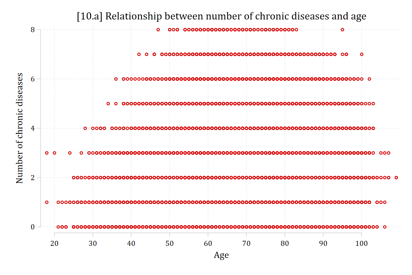
// 10.a - Basic scatterplot doesn't work because of overlapping data points
twoway scatter dzcount age, ///
    title("[10.a] Relationship between number of chronic diseases and age") //
/
    xtitle("Age") ytitle("Number of chronic diseases") ///
    xlabel(20(10)100)

[10.a] Scatterplot of the number of chronic diseases (0 to 8) by age: because both variables take whole-number values, the points overlap into solid horizontal rows, and the graph cannot show where most of the data are.

library(foreign)            # load Stata datasets
library(ggplot2)            # main graphics package
library(dplyr)              # data manipulation tools
library(cleanplots)         # Mize's graphics scheme

## Use cleanplots colors, markers, lines, and theme for all graphs ##
cleanplots_defaults()
theme_update(plot.title.position = "plot")   # titles start at left edge of graph

# Health and Retirement Study Data
hrs <- read.dta("https://tdmize.github.io/data/data/hrs_si.dta")

# 10.a - Basic scatterplot doesn't work because of overlapping data points
ggplot(hrs, aes(x = age, y = dzcount)) +
  geom_point() +
  labs(x = "Age",
       y = "Number of chronic diseases",
       title = "[10.a] Relationship between number of chronic diseases and age") +
  scale_x_continuous(breaks = seq(20, 100, 10))
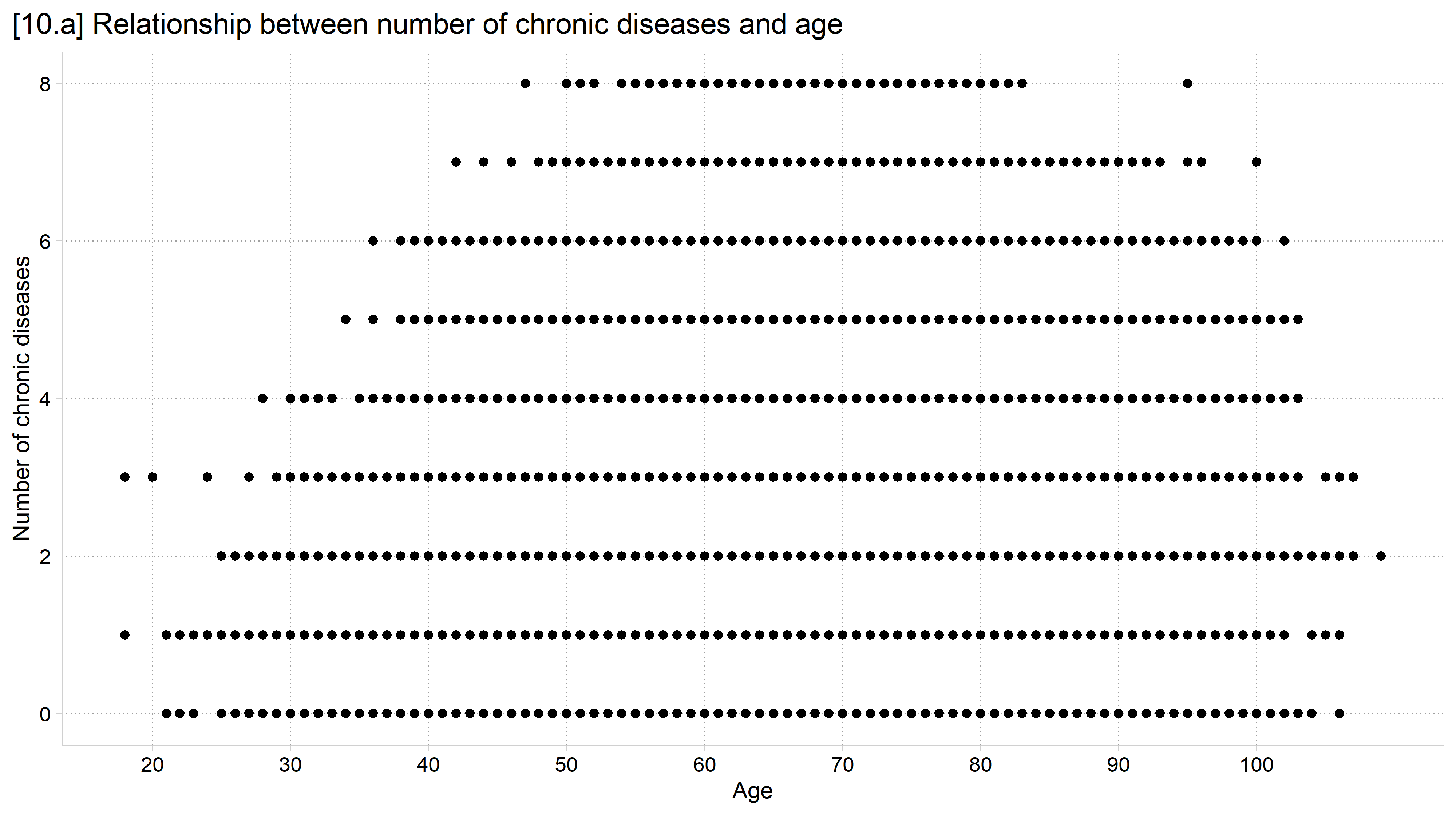
[10.a] Scatterplot of the number of chronic diseases (0 to 8) by age: because both variables take whole-number values, the points overlap into solid horizontal rows, and the graph cannot show where most of the data are.

// 10.b - Jitter (random noise) points to prevent overlap
twoway scatter dzcount age, jitter(3) ///
    title("[10.b] Relationship between number of chronic diseases and age") //
/
    subtitle("Data points have been jittered to prevent overlap") ///
    xtitle("Age") ytitle("Number of chronic diseases") ///
    xlabel(20(10)100)

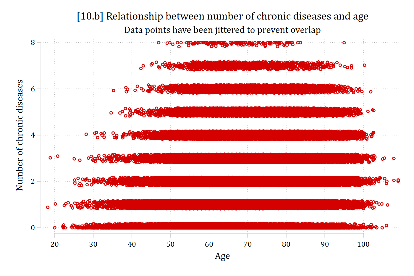
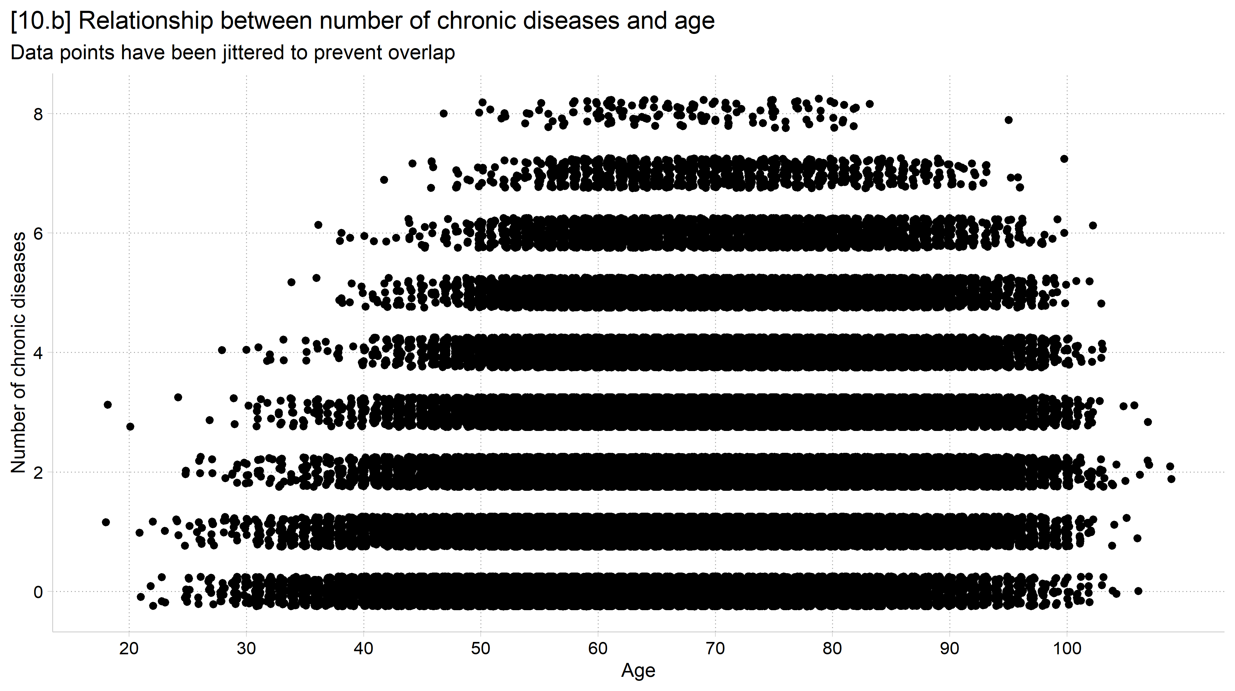
[10.b] The same scatterplot with random noise added to each point: the rows become thick bands, showing that most observations are between ages 50 and 95, but with so many points the bands are still solid.

# 10.b - Jitter (random noise) points to prevent overlap
ggplot(hrs, aes(x = age, y = dzcount)) +
  geom_jitter(height = .25, width = .25) +
  labs(x = "Age",
       y = "Number of chronic diseases",
       title = "[10.b] Relationship between number of chronic diseases and age",
       subtitle = "Data points have been jittered to prevent overlap") +
  scale_x_continuous(breaks = seq(20, 100, 10))
[10.b] The same scatterplot with random noise added to each point: the rows become thick bands, showing that most observations are between ages 50 and 95, but with so many points the bands are still solid.

Binned scatterplots

  • Scatterplots and scatterplot smoothing methods like lowess are less useful when you have lots of data
    • Graphs become impossible to read (but could plot random subsample)
  • A binned scatterplot is a useful tool for these and other cases (Stepner 2014)
    • “bin” the x variable into groups (e.g., 20 age groups) and then calculate the mean of the y variable for each bin
// 10.c - Binned scatterplot: mean of y within 20 equal-sized bins of x
binscatter dzcount age, linetype(none) mcolors(red*1.2) ///
    title("[10.c] Binned scatterplot for number of chronic diseases by age") /
//
    subtitle("Each point is the mean in one of 20 equal-sized age groups") ///
    xtitle("Age") ytitle("Number of chronic diseases") ///
    xlabel(20(10)100)

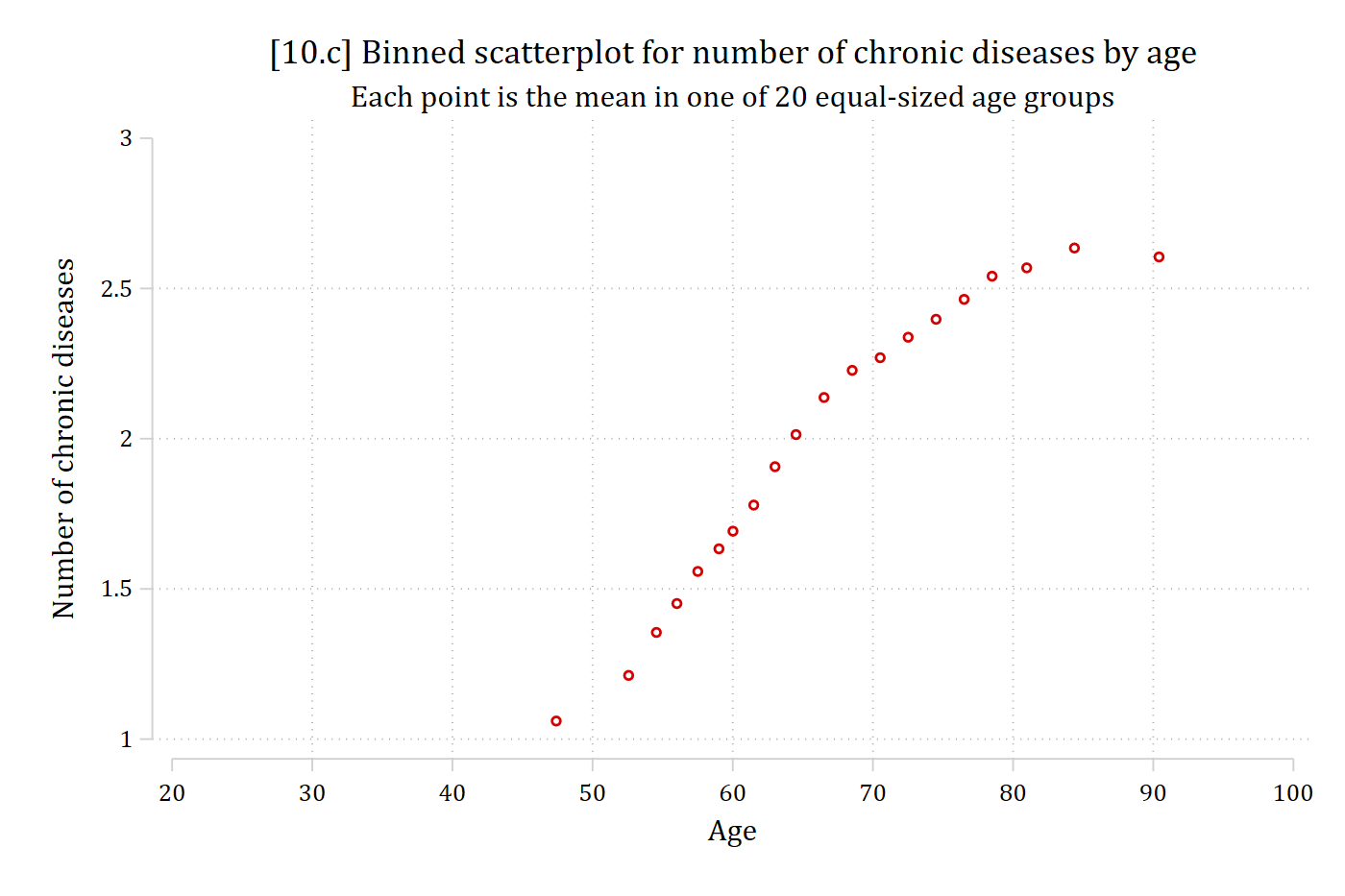
[10.c] Binned scatterplot with one point for the mean number of chronic diseases in each of 20 equal-sized age groups: the mean rises steeply from about 1 at age 47 to about 2.3 at age 70 and then levels off near 2.6 after age 80.

# 10.c - Binned scatterplot: mean of y within 20 equal-sized bins of x
hrs_bins <- hrs %>%
  filter(!is.na(dzcount), !is.na(age)) %>%
  mutate(age_bin = ntile(age, 20)) %>%
  group_by(age_bin) %>%
  summarise(age = mean(age), dzcount = mean(dzcount))

ggplot(hrs_bins, aes(x = age, y = dzcount)) +
  geom_point(size = 3) +
  labs(x = "Age",
       y = "Number of chronic diseases",
       title = "[10.c] Binned scatterplot for number of chronic diseases by age",
       subtitle = "Each point is the mean in one of 20 equal-sized age groups") +
  scale_x_continuous(breaks = seq(20, 100, 10))
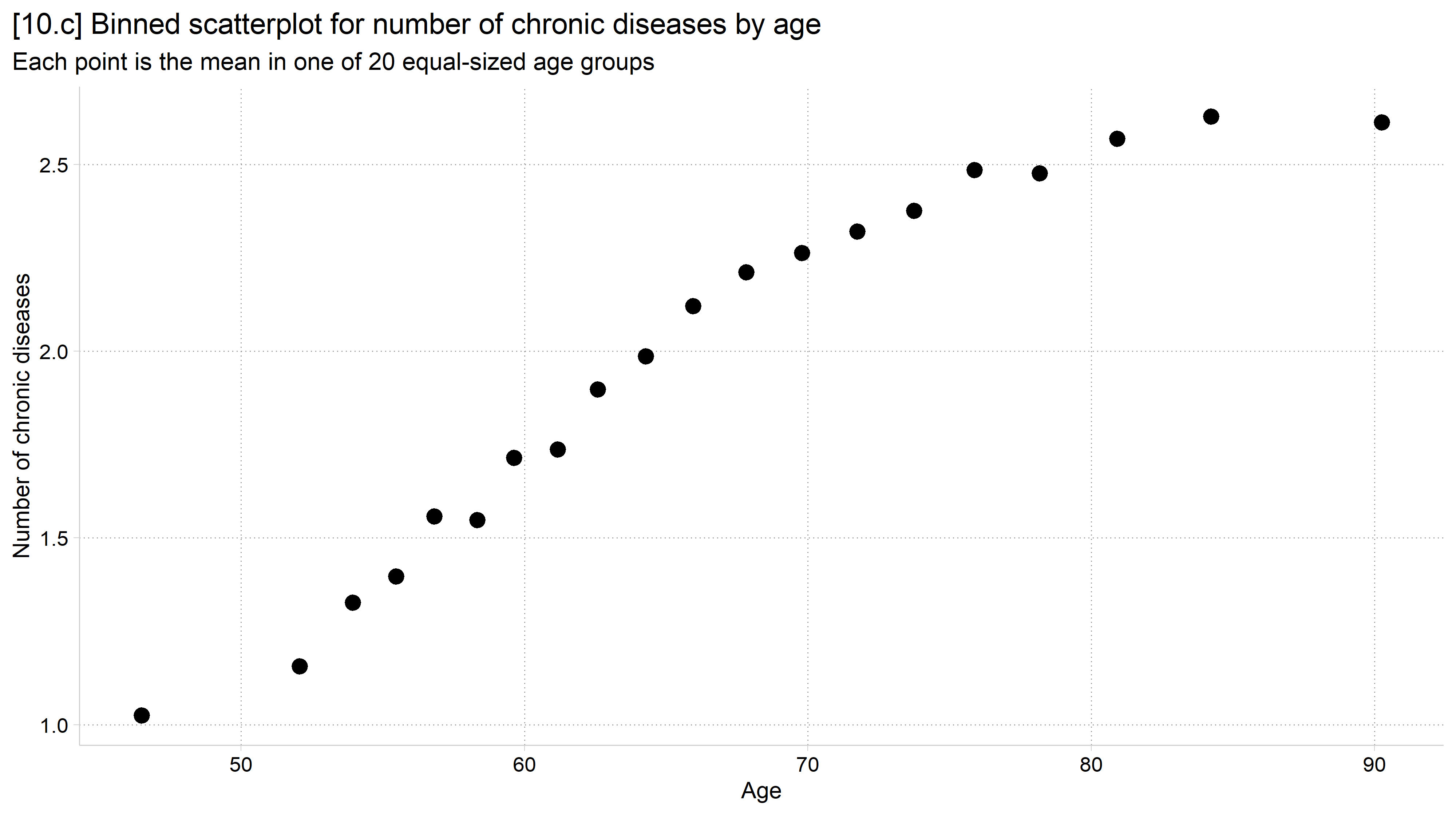
[10.c] Binned scatterplot with one point for the mean number of chronic diseases in each of 20 equal-sized age groups: the mean rises steeply from about 1 near age 47 and then levels off after age 80.

// 10.d - Linear regression line overlaid on scatterplot
twoway ///
    (scatter dzcount age, jitter(3) mcolor(gs12)) ///
    (lfit dzcount age, lcolor(red)), ///
    legend(off) xlabel(20(10)100) ///
    title("[10.d] Relationship between number of chronic diseases and age") //
/
    subtitle("With linear trend line") ///
    xtitle("Age") ytitle("Number of chronic diseases")

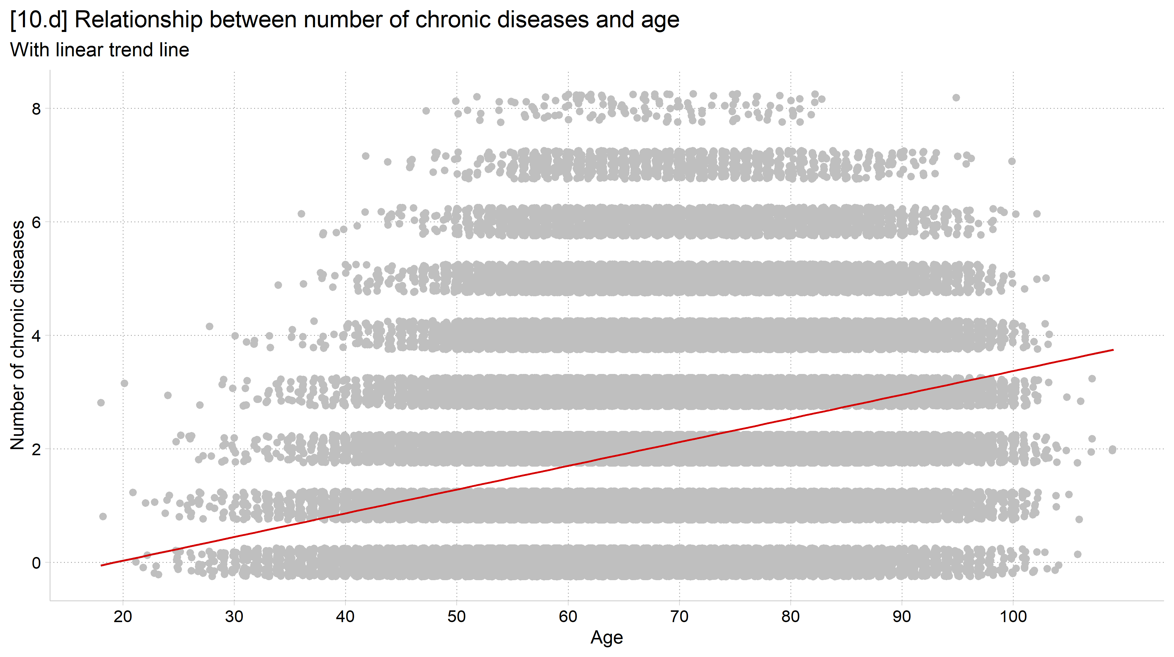
[10.d] The jittered scatterplot in light gray with a red linear regression line that rises steadily with age across the whole range.

# 10.d - Linear regression line overlaid on scatterplot
ggplot(hrs, aes(x = age, y = dzcount)) +
  geom_jitter(height = .25, width = .25, color = "gray75") +
  geom_smooth(method = "lm") +
  labs(x = "Age",
       y = "Number of chronic diseases",
       title = "[10.d] Relationship between number of chronic diseases and age",
       subtitle = "With linear trend line") +
  scale_x_continuous(breaks = seq(20, 100, 10))
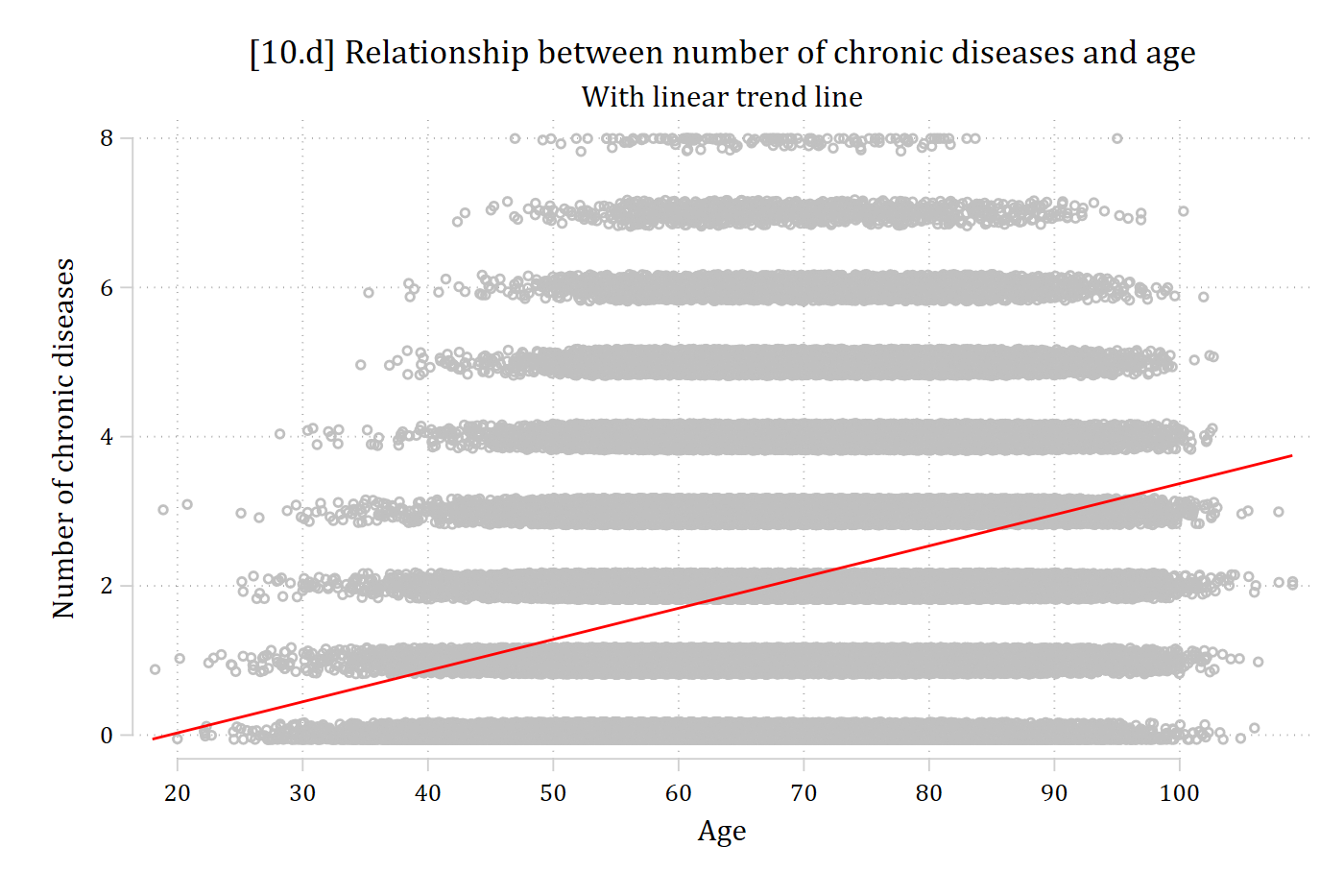
[10.d] The jittered scatterplot in light gray with a linear regression line that rises steadily with age across the whole range.

// 10.e - Quadratic regression line (x and x^2) overlaid on scatterplot
twoway ///
    (scatter dzcount age, jitter(2) mcolor(gs12)) ///
    (qfit dzcount age, lcolor(red)), ///
    legend(off) xlabel(20(10)100) ///
    title("[10.e] Relationship between number of chronic diseases and age") //
/
    subtitle("With quadratic trend line") ///
    xtitle("Age") ytitle("Number of chronic diseases")

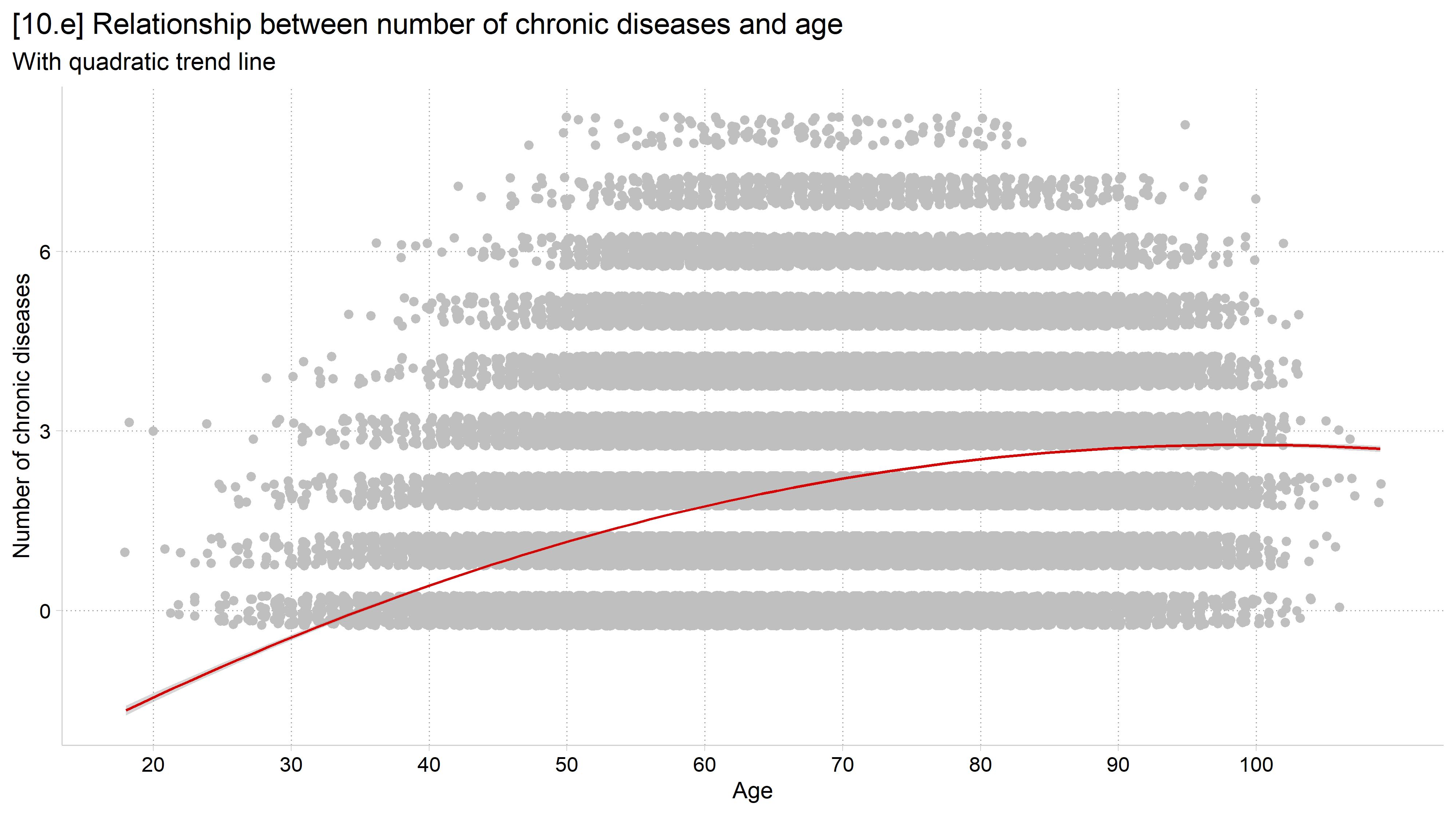
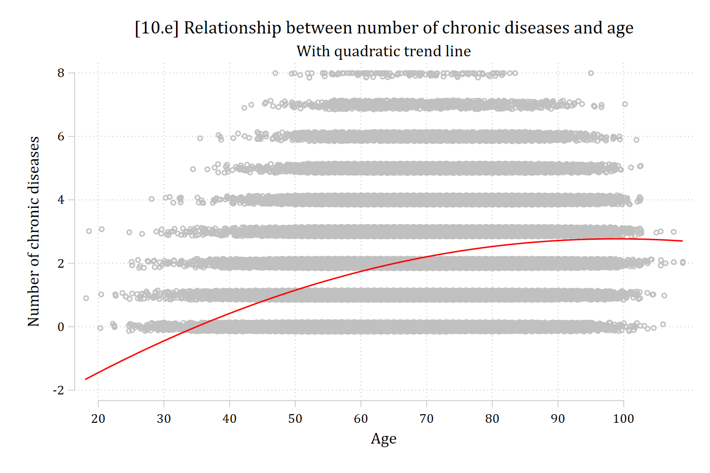
[10.e] The jittered scatterplot with a red quadratic regression line that rises with age and flattens out at the oldest ages.

# 10.e - Quadratic regression line (x and x^2) overlaid on scatterplot
ggplot(hrs, aes(x = age, y = dzcount)) +
  geom_jitter(height = .25, width = .25, color = "gray75") +
  geom_smooth(method = "lm", formula = y ~ poly(x, 2)) +
  labs(x = "Age",
       y = "Number of chronic diseases",
       title = "[10.e] Relationship between number of chronic diseases and age",
       subtitle = "With quadratic trend line") +
  scale_x_continuous(breaks = seq(20, 100, 10))
[10.e] The jittered scatterplot with a quadratic regression line that rises with age and flattens out at the oldest ages.

LOWESS: locally weighted scatterplot smoothing

  • The fitted lines shown above are parametric techniques
  • LOWESS performs “local” regressions on a subset of your data
    • Primarily an exploratory technique—you can plot the smoothed regression line but you do not get parameter estimates/significance tests
    • It can be a helpful way to quickly assess nonlinearity and often suggests possible parametric modeling solutions for the nonlinearity (e.g., need both age and age2 in model)
  • Can specify a bandwidth (bwidth( ) option in Stata; span in R) to determine how much to smooth (0 to 1 as a proportion of your data)
    • E.g., A bandwidth of 0.4 means you want the 40% of the data closest to a given point used to calculate the line at that point
    • Smaller bandwidths will let you find more nonlinearities but are more susceptible to outliers and other quirks of your data
      • I find 0.3 or 0.4 good starting places
// 10.f - Lowess smoothed fit line (2022 wave only)
twoway ///
    (scatter dzcount age if year == 2022, jitter(2) mcolor(gs12)) ///
    (lowess dzcount age if year == 2022, bwidth(.4) lcolor(red)), ///
    legend(off) xlabel(20(10)100) ///
    title("[10.f] Relationship between number of chronic diseases and age") //
/
    subtitle("With lowess trend line (bandwidth = 0.4)") ///
    xtitle("Age") ytitle("Number of chronic diseases")

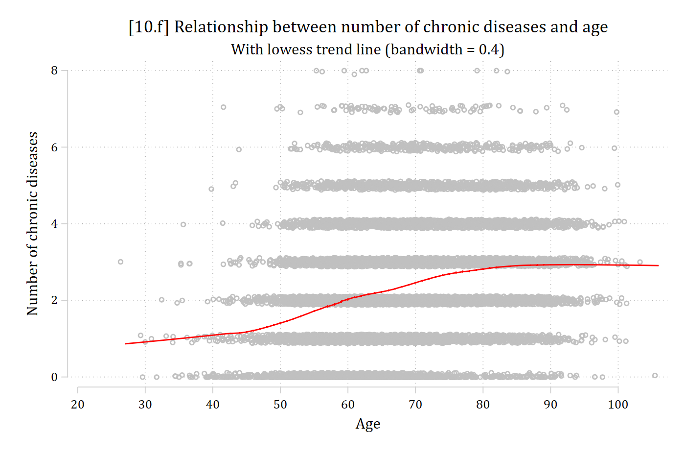
[10.f] Jittered scatterplot of chronic diseases by age for the 2022 wave with a red lowess line: the line is nearly flat around 1 until about age 45, rises between 45 and 80, and levels off near 3 after age 80.

# 10.f - Lowess smoothed fit line (2022 wave only)
ggplot(filter(hrs, year == 2022), aes(x = age, y = dzcount)) +
  geom_jitter(height = .25, width = .25, color = "gray75") +
  geom_smooth(method = "loess", se = FALSE, span = .4) +
  labs(x = "Age",
       y = "Number of chronic diseases",
       title = "[10.f] Relationship between number of chronic diseases and age",
       subtitle = "With lowess trend line (span = 0.4)") +
  scale_x_continuous(breaks = seq(20, 100, 10))
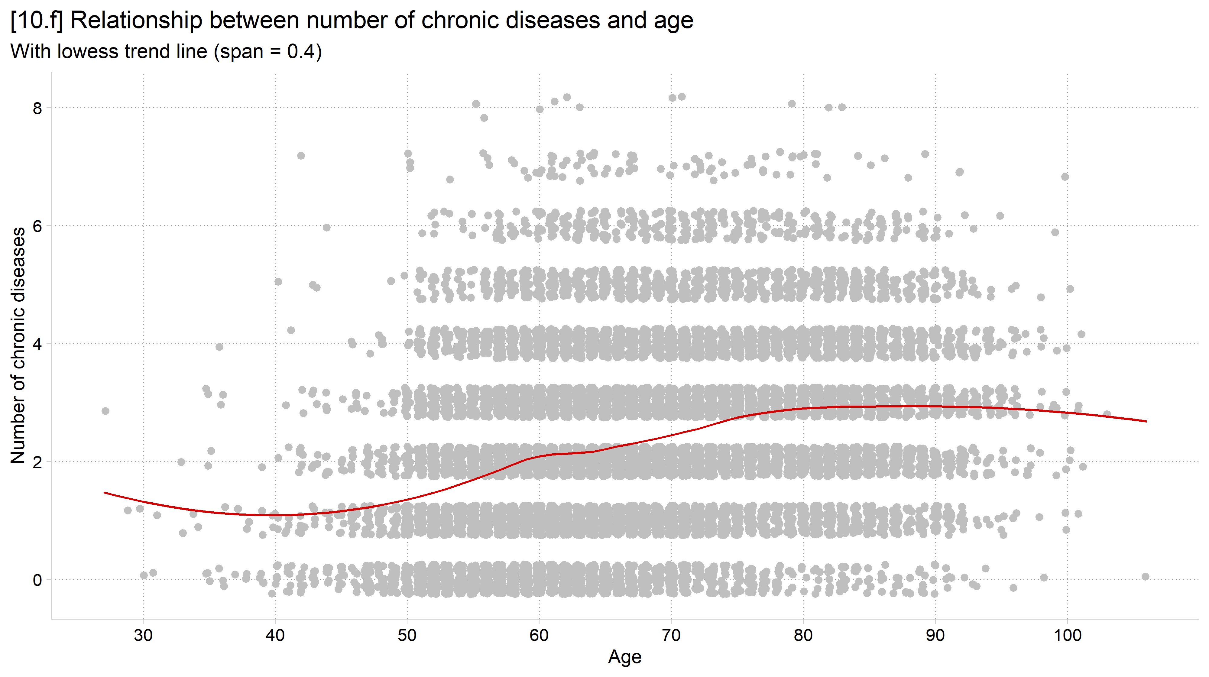
[10.f] Jittered scatterplot of chronic diseases by age for the 2022 wave with a lowess line: the line is nearly flat until about age 45, rises between 45 and 80, and levels off after age 80.

Published example

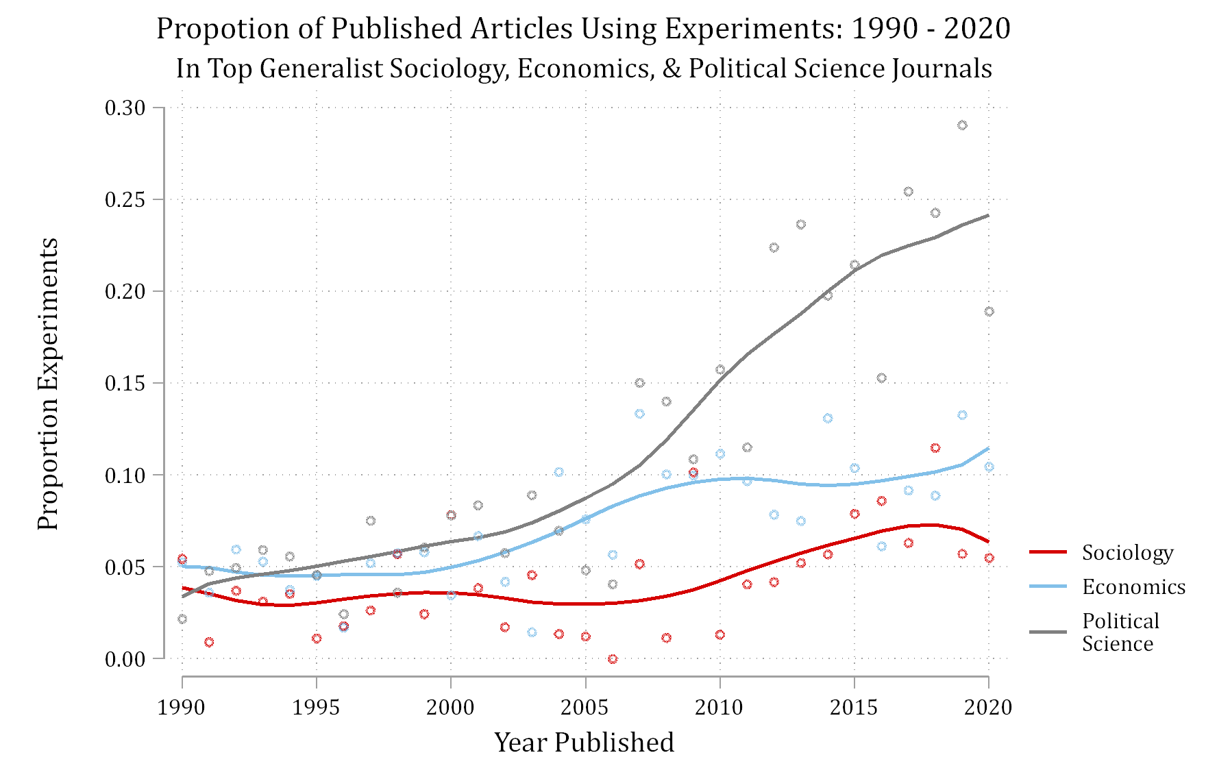
Published figure: the proportion of published articles using experiments from 1990 to 2020 in top generalist sociology, economics, and political science journals, with smoothed trend lines for each field.

*Figure 1 from Mize and Manago 2022

Historical example

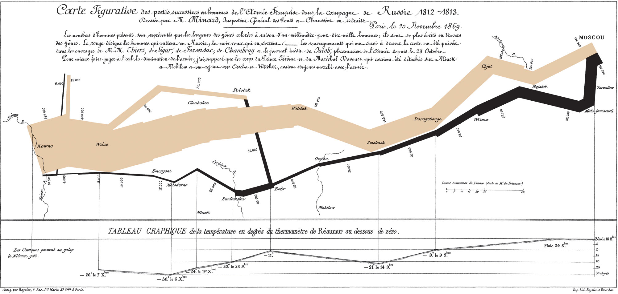
Napoleon’s march to, and retreat from, Moscow in the War of 1812

Charles Minard's 1869 chart of Napoleon's march to and retreat from Moscow: a tan band for the army's advance and a black band for its retreat, whose widths show the shrinking size of the army, with a temperature line below.

*Read more about the graphic here

The Methodology Center illustration: small line drawings of graphs around a central MCAP circle.

Minard's chart of Napoleon's march, which one of the drawings in the Methodology Center illustration is based on.

*Read about The Methodology Center graphic

Back to top