3.9 Risk Ratios/Relative Risk (RR)

Calculating risk ratios

  • Recall the formula for the marginal effect at the mean (MEM):

\[MEM = \eta(x_{k} = end, \mathbf{x} = \overline{\mathbf{x}}) - \eta(x_{k} = start, \mathbf{x} = \overline{\mathbf{x}})\]

  • For the MEM, we are subtracting a prediction at an ending value from a prediction at a starting value
  • A risk ratio (RR) simply quantifies the effect in terms of a ratio of ending/starting values rather than a difference (as the MEM or AME does)*

\[RR = \frac{\eta(x_{k} = end, \mathbf{x} = \mathbf{x}^{*})}{\eta(x_{k} = start, \mathbf{x} = \mathbf{x}^{*})}\]

  • Risk ratios are generally used to interpret group differences (e.g., men compared to women; participants in the treatment condition compared to participants in the control condition; etc.)
    • Below, I represent the grouping variable as g (which equals 0 or 1)

\[RR = \frac{\eta(g = 1, \mathbf{x} = \mathbf{x}^{*})}{\eta(g = 0, \mathbf{x} = \mathbf{x}^{*})}\]

*Note we have the same options here as with marginal effects for what to do with the covariates in x*

Risk ratio example: cognition among older adults

  • Risk ratios most often used in health research (hence “risk” terminology)
  • Health and Retirement Study data (older adults) from 2020
    • DV: Very low, dementia level score on cognitive test (0/1)
// Health and Retirement Study 2020
use "https://tdmize.github.io/data/data/cda_hrs", clear
(cda_hrs.dta | Health & Retirement Study 2020)
drop if missing(cogB, marstatB, collegeB, woman, age, nlivsib)
(774 observations deleted)
fre cogB marstatB
cogB -- Dementia-range cognition
-----------------------------------------------------------
              |      Freq.    Percent      Valid       Cum.
--------------+--------------------------------------------
Valid   0 no  |      14366      96.10      96.10      96.10
        1 yes |        583       3.90       3.90     100.00
        Total |      14949     100.00     100.00           
-----------------------------------------------------------

marstatB -- Currently married
-----------------------------------------------------------------------------
                                |      Freq.    Percent      Valid       Cum.
--------------------------------+--------------------------------------------
Valid   0 not currently married |       5863      39.22      39.22      39.22
        1 currently married     |       9086      60.78      60.78     100.00
        Total                   |      14949     100.00     100.00           
-----------------------------------------------------------------------------
rename marstatB married
library(haven)           # import Stata data and labels
library(dplyr)           # data manipulation
library(sjmisc)          # frequency tables
library(marginaleffects) # predictions and marginal effects

# Health and Retirement Study 2020
hrs <- read_dta("https://tdmize.github.io/data/data/cda_hrs.dta")

hrs <- hrs[complete.cases(hrs[c("cogB", "marstatB", "collegeB", "woman", "age",
  "nlivsib")]), ]
frq(hrs, cogB, marstatB)
Dementia-range cognition (cogB) <numeric> 
# total N=14949 valid N=14949 mean=0.04 sd=0.19

Value | Label |     N | Raw % | Valid % | Cum. %
------------------------------------------------
    0 |    no | 14366 | 96.10 |   96.10 |  96.10
    1 |   yes |   583 |  3.90 |    3.90 | 100.00
 <NA> |  <NA> |     0 |  0.00 |    <NA> |   <NA>

Currently married (marstatB) <numeric> 
# total N=14949 valid N=14949 mean=0.61 sd=0.49

Value |                 Label |    N | Raw % | Valid % | Cum. %
---------------------------------------------------------------
    0 | not currently married | 5863 | 39.22 |   39.22 |  39.22
    1 |     currently married | 9086 | 60.78 |   60.78 | 100.00
 <NA> |                  <NA> |    0 |  0.00 |    <NA> |   <NA>
hrs <- hrs |> rename(married = marstatB)
  • IVs:
    • Focal: college degree (0/1)
    • Controls: married, woman, age
* Predict dementia level poor cognition binary
logit cogB i.collegeB i.married i.woman c.age, or
Iteration 0:  Log likelihood = -2462.8569  
Iteration 1:  Log likelihood = -2308.2881  
Iteration 2:  Log likelihood = -2279.0977  
Iteration 3:  Log likelihood = -2278.6349  
Iteration 4:  Log likelihood = -2278.6335  
Iteration 5:  Log likelihood = -2278.6335  

Logistic regression                                     Number of obs = 14,949
                                                        LR chi2(4)    = 368.45
                                                        Prob > chi2   = 0.0000
Log likelihood = -2278.6335                             Pseudo R2     = 0.0748

-------------------------------------------------------------------------------
         cogB | Odds ratio   Std. err.      z    P>|z|     [95% conf. interval]
--------------+----------------------------------------------------------------
     collegeB |
bachelor's..  |      0.233      0.037   -9.254   0.000        0.171       0.317
              |
      married |
currently ..  |      0.554      0.051   -6.430   0.000        0.463       0.664
              |
        woman |
       woman  |      0.805      0.073   -2.379   0.017        0.673       0.962
          age |      1.049      0.004   12.079   0.000        1.041       1.057
        _cons |      0.003      0.001  -19.121   0.000        0.001       0.005
-------------------------------------------------------------------------------
Note: _cons estimates baseline odds.
est store cogmod
# Treat binary variables as factors using their value labels
hrs <- hrs |>
  mutate(collegeB = as_factor(collegeB), married = as_factor(married),
    woman = as_factor(woman))

# Predict dementia level poor cognition binary
cogmod <- glm(cogB ~ collegeB + married + woman + age,
  family = binomial(link = "logit"), data = hrs)
summary(cogmod)

Call:
glm(formula = cogB ~ collegeB + married + woman + age, family = binomial(link = "logit"), 
    data = hrs)

Coefficients:
                              Estimate Std. Error z value Pr(>|z|)    
(Intercept)                  -5.928818   0.310060 -19.121  < 2e-16 ***
collegeBbachelor's or higher -1.455602   0.157298  -9.254  < 2e-16 ***
marriedcurrently married     -0.589861   0.091729  -6.430 1.27e-10 ***
womanwoman                   -0.216973   0.091190  -2.379   0.0173 *  
age                           0.048089   0.003981  12.079  < 2e-16 ***
---
Signif. codes:  0 '***' 0.001 '**' 0.01 '*' 0.05 '.' 0.1 ' ' 1

(Dispersion parameter for binomial family taken to be 1)

    Null deviance: 4925.7  on 14948  degrees of freedom
Residual deviance: 4557.3  on 14944  degrees of freedom
AIC: 4567.3

Number of Fisher Scoring iterations: 7
  • First, make predictions for each category of the binary/nominal IV
* Risk ratio, averaging over observed values
est restore cogmod
(results cogmod are active now)
margins collegeB, post
Predictive margins                                      Number of obs = 14,949
Model VCE: OIM

Expression: Pr(cogB), predict()

-------------------------------------------------------------------------------
              |            Delta-method
              |     Margin   std. err.      z    P>|z|     [95% conf. interval]
--------------+----------------------------------------------------------------
     collegeB |
no bachelo..  |      0.048      0.002   23.964   0.000        0.044       0.052
bachelor's..  |      0.012      0.002    6.758   0.000        0.008       0.015
-------------------------------------------------------------------------------
avg_predictions(cogmod, variables = "collegeB", by = "collegeB")

             collegeB Estimate Std. Error     z Pr(>|z|)     S   2.5 % 97.5 %
 no bachelor's          0.0482    0.00201 23.96   <0.001 419.2 0.04428 0.0522
 bachelor's or higher   0.0119    0.00176  6.76   <0.001  36.1 0.00844 0.0153

Type: response

Older adults without a college degree have a 0.048 probability of having very low dementia-level cognition, compared to only a 0.012 probability for older adults with college degree

  • MEs and RRs are based on same information (two predicted probabilities)
    • One subtracts the two (MEs)
    • One divides them to get the multiplicative effect (RR)
* Replicate mecompare's AME
metest 1 - 2
                                 |  estimate         se     pvalue 
---------------------------------+--------------------------------
       0bn_collegeB - 1_collegeB |     0.036      0.003      0.000 
# no bachelor's - bachelor's or higher
avg_predictions(cogmod, variables = "collegeB", by = "collegeB",
  hypothesis = ~ revpairwise)

                               Hypothesis Estimate Std. Error    z Pr(>|z|)     S  2.5 % 97.5 %
 (no bachelor's) - (bachelor's or higher)   0.0363    0.00268 13.6   <0.001 136.8 0.0311 0.0416

Type: response

This replicates what mecompare and avg_comparisons calculates

AME: Older adults without college degrees have a 0.036 higher probability of having very low dementia-level cognition than do older adults with a college degree

* Compute risk ratio with metest, which # refers to row of prediction
metest 1 / 2
                                 |  estimate         se     pvalue 
---------------------------------+--------------------------------
       0bn_collegeB / 1_collegeB |     4.056      0.624      0.000 
# no bachelor's / bachelor's or higher
avg_predictions(cogmod, variables = "collegeB", by = "collegeB",
  hypothesis = ratio ~ revpairwise)

                               Hypothesis Estimate Std. Error    z Pr(>|z|)    S 2.5 % 97.5 %
 (no bachelor's) / (bachelor's or higher)     4.06      0.624 4.89   <0.001 20.0  2.83   5.28

Type: response

RR: The risk of having dementia-level cognition is 4.056 times higher for older adults without a college degree

Should you use MEs or risk ratios (RRs)?

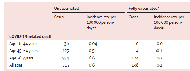
  • This example from Haas et al. 2021 which tracked COVID cases and deaths in Israel after widespread availability of the Pfizer vaccine
    • DV: COVID-19 related deaths
    • IV: Vaccinated or not (assume roughly equal #s in each group for simplicity)
    • IV: Data is divided into three age strata: 16 - 44, 45 - 64, and 65+

COVID-19-related death rows of Table 2 from Haas et al. (2021): COVID-19-related deaths among unvaccinated and fully vaccinated people by age group: 36 versus 0 deaths for ages 16 to 44, 125 versus 14 for ages 45 to 64, 554 versus 124 for ages 65 and older, and 715 versus 138 for all ages.

*Table 2 from Haas et al. 2021

Vaccine efficacy (RRs)

  • What is vaccine efficacy against death?
    • Simplest calculation is what % of deaths were among the unvaccinated

\[{efficacy}_{16-44} = 1 - \frac{0}{0 + 36} \approx 100\%\]

\[{efficacy}_{45-64} = 1 - \frac{14}{14 + 125} \approx 89.93\%\]

\[{efficacy}_{65+} = 1 - \frac{124}{124 + 554} \approx 81.71\%\]

  • How effective is the vaccine? If you are young, it reduces your chance of dying from COVID by approximately 100%
    • It is less effective at preventing death for older adults
    • These are risk ratios
      • They are useful for determining if a vaccine works and how effective it is among different groups

Risk difference (ME) for COVID death

  • But how many people did the vaccine prevent from dying?
    • Calculate the simple difference in deaths across each group

\[{deaths\ prevented}_{16-44} = 36 - 0 = 36\]

\[{deaths\ prevented}_{45-64} = 125 - 14 = 111\]

\[{deaths\ prevented}_{65+} = 554 - 124 = 430\]

  • About 111 people 45 - 64 years old died unnecessarily: their deaths could have been prevented by getting vaccinated
    • This risk difference is a marginal effect as it calculates the difference in deaths for each age group

Should you use the marginal effect (ME) or risk ratio (RR)?

  • Refer back to the results above
    • The vaccine is more efficacious for younger people
    • Despite being less efficacious for older people, the vaccine prevents far more deaths among older people than among younger people
  • The RR and ME point in opposite directions about the vaccine’s effect based on age
    • Why? Base rates of deaths are much higher for older people
  • Given this conflicting evidence, which would you use?
    • If you were in charge of giving out the first vaccines, when they were still limited, who would you prioritize access for?
      • Older or younger adults?
      • Why?
  • Do you want to decide if the vaccine works and whether it should be approved?
    • Use the RR
  • Do you want to help the most people?
    • E.g., Who should you give the first available doses to?
      • Use the ME: prioritizing older people getting vaccinated will prevent the most deaths despite the fact the efficacy RR is lower for older people

More thoughts on risk ratios

“For each set of 100,000 people who have one drink a day per year, 918 can expect to experience one of the 23 alcohol-related problems in any year. Of those who drink nothing, 914 can expect to experience a problem. This means that 99,082 are unaffected, and 914 will have an issue no matter what. Only 4 in 100,000 people who consume a drink a day may have a problem caused by the drinking, according to this study.” (Carroll 2018)

  • Recall the NY Times Upshot article about the risk of alcohol-related diseases based on # of drinks consumed
    • A large risk ratio does not necessarily translate into a large number of people affected

Ina Garten holding a cocktail shaker and a cocktail.

Ina Garten drinking from an enormous cocktail glass.

More thoughts on RRs vs MEs

  • RR effect sizes are harder to understand and often misinterpreted
    • Because negative effects are bounded between 0 and 1, easy to misunderstand effect size
      • E.g., 20 is the same size RR as 0.05 just in the opposite direction
    • There is an upper bound on effect size for common but not rare outcomes
  • Sometimes a multiplicate effect may be of theoretical/substantive interest—in this case, I would recommend using an RR instead of relying on the odds ratio (OR)
    • I would only consider RRs for summaries of an effect (e.g., to replace ORs in a regression table)
  • I find it odd that many scholars argue for multiplicative effects only with binary DVs
    • We can calculate multiplicative effects in linear models—but this is rarely done
  • Here, a linear model using HRS that predicts # of siblings (which is really a count)
// Show a risk ratio calculation in linear model
regress nlivsib i.collegeB i.married i.woman c.age
      Source |       SS           df       MS      Number of obs   =    14,949
-------------+----------------------------------   F(4, 14944)     =    229.64
       Model |  6163.72331         4  1540.93083   Prob > F        =    0.0000
    Residual |  100278.753    14,944  6.71030201   R-squared       =    0.0579
-------------+----------------------------------   Adj R-squared   =    0.0577
       Total |  106442.477    14,948  7.12085072   Root MSE        =    2.5904

-------------------------------------------------------------------------------
      nlivsib | Coefficient  Std. err.      t    P>|t|     [95% conf. interval]
--------------+----------------------------------------------------------------
     collegeB |
bachelor's..  |     -1.030      0.048  -21.400   0.000       -1.125      -0.936
              |
      married |
currently ..  |     -0.088      0.045   -1.944   0.052       -0.177       0.001
              |
        woman |
       woman  |      0.055      0.044    1.231   0.218       -0.032       0.141
          age |     -0.043      0.002  -21.193   0.000       -0.047      -0.039
        _cons |      6.632      0.152   43.665   0.000        6.334       6.930
-------------------------------------------------------------------------------
# Show a risk ratio calculation in linear model
sibmod <- lm(nlivsib ~ collegeB + married + woman + age, data = hrs)
summary(sibmod)

Call:
lm(formula = nlivsib ~ collegeB + married + woman + age, data = hrs)

Residuals:
    Min      1Q  Median      3Q     Max 
-5.0456 -1.8583 -0.5995  1.1623 20.3766 

Coefficients:
                              Estimate Std. Error t value Pr(>|t|)    
(Intercept)                   6.632177   0.151889  43.665   <2e-16 ***
collegeBbachelor's or higher -1.030352   0.048146 -21.400   <2e-16 ***
marriedcurrently married     -0.088087   0.045310  -1.944   0.0519 .  
womanwoman                    0.054502   0.044283   1.231   0.2184    
age                          -0.043139   0.002036 -21.193   <2e-16 ***
---
Signif. codes:  0 '***' 0.001 '**' 0.01 '*' 0.05 '.' 0.1 ' ' 1

Residual standard error: 2.59 on 14944 degrees of freedom
Multiple R-squared:  0.05791,   Adjusted R-squared:  0.05765 
F-statistic: 229.6 on 4 and 14944 DF,  p-value: < 2.2e-16

Coefficient / ME: Older adults with college degrees have about one fewer sibling than do older adults without college degrees

* Risk ratio, averaging over observed values
margins collegeB, post
Predictive margins                                      Number of obs = 14,949
Model VCE: OLS

Expression: Linear prediction, predict()

-------------------------------------------------------------------------------
              |            Delta-method
              |     Margin   std. err.      t    P>|t|     [95% conf. interval]
--------------+----------------------------------------------------------------
     collegeB |
no bachelo..  |      3.693      0.025  148.948   0.000        3.644       3.741
bachelor's..  |      2.662      0.041   64.700   0.000        2.582       2.743
-------------------------------------------------------------------------------
avg_predictions(sibmod, variables = "collegeB", by = "collegeB")

             collegeB Estimate Std. Error     z Pr(>|z|)   S 2.5 % 97.5 %
 no bachelor's            3.69     0.0248 148.9   <0.001 Inf  3.64   3.74
 bachelor's or higher     2.66     0.0411  64.7   <0.001 Inf  2.58   2.74

Type: response
  • We can calculate a risk ratio in a linear model just as with a binary model by dividing the predictions
* Compute risk ratio with metest, which # refers to row of prediction
metest 2 / 1
                                 |  estimate         se     pvalue 
---------------------------------+--------------------------------
       1_collegeB / 0bn_collegeB |     0.721      0.012      0.000 
# bachelor's or higher / no bachelor's
avg_predictions(sibmod, variables = "collegeB", by = "collegeB",
  hypothesis = ratio ~ pairwise)

                               Hypothesis Estimate Std. Error     z Pr(>|z|)     S 2.5 % 97.5 %
 (bachelor's or higher) / (no bachelor's)    0.721     0.0122 -22.9   <0.001 384.0 0.697  0.745

Type: response

Risk ratio: Older adults with college degrees have about 0.72 times fewer siblings than do older adults without college degrees

Cartoon of a confused person surrounded by question marks.

  • In general, I find graphs of predicted probabilities and marginal effects to be more helpful, more easily interpretable, and more satisfying summaries of effects
  • Marginal effects summarize effects in an intuitive and additive metric
    • MEs are the most similar method of interpretation to how the coefficients are interpreted in linear regression so the most familiar/easiest for most people to understand
    • Effect size is also easier to understand, as the impact of a multiplicative effect (e.g., OR or RR) is dependent on the starting point / base rate
Star Wars meme: NEVER TELL ME THE RATIOS.

Back to top