Think about the substantive issue your model is describing. What types of people are you interested in? What are interesting clusters of characteristics about your observations? That is, what combined values of multiple IVs represent interesting/important “types” of people to examine?
These sets of characteristics are called ideal types or profiles (“ideal type” from Max Weber)
“Ideal type: a common mental construct in the social sciences derived from observable reality although not conforming to it in detail because of deliberate simplification and exaggeration. It is not ideal in the sense that it is excellent, nor is it an average; it is, rather, a constructed ideal used to approximate reality by selecting and accentuating certain elements.”
Pr(Trump) for Various Ideal Types of Voters

Expression: Pr(trump), predict()

                 |    Pr(y)
 ----------------+---------
         Average |    0.440
        MAGA Man |    0.608
    Romney Repub |    0.434
        Dem Base |    0.061

Specified values where .n indicates no values specified with at()

           |  No at()     woman       age      educ      race    income
 ----------+------------------------------------------------------------
     Set 1 |       .n         .         .         .         .         .
     Set 2 |        .         0        70         2         1        30
     Set 3 |        .         0        40         4         1       150
   Current |        .         1        30         4         2        50

           |   region
 ----------+---------
     Set 1 |        .
     Set 2 |        2
     Set 3 |        1
   Current |        4
library(haven) # import Stata data and labelslibrary(dplyr) # data manipulationlibrary(marginaleffects) # predictions and marginal effects# 2016 US Election Datapew <-read_dta("https://tdmize.github.io/data/data/cda_pew.dta")# Recode data for example; treat binary/nominal variables as factorspew <- pew |>mutate(trump =as.numeric(presvote2),religB =factor(if_else(relattend >=4, "Religious", "Not Religious")),woman =as_factor(woman), educ =as_factor(educ), race =as_factor(race),polparty3 =as_factor(polparty3), region =as_factor(region),clintongend =as_factor(clintongend), student =as_factor(student),polviews =as_factor(polviews)) |>droplevels()trumpmod <-glm(trump ~ woman + age + educ + race + polparty3 + religB + income + region,family =binomial(link ="logit"), data = pew)summary(trumpmod)
Call:
glm(formula = trump ~ woman + age + educ + race + polparty3 +
    religB + income + region, family = binomial(link = "logit"),
    data = pew)

Coefficients:
                      Estimate Std. Error z value Pr(>|z|)
(Intercept)           1.128548   0.728631   1.549  0.12142
womanWoman           -0.522591   0.173407  -3.014  0.00258 **
age                   0.013823   0.005193   2.662  0.00777 **
educHS Degree         1.461868   0.651509   2.244  0.02484 *
educSome College      0.677411   0.643354   1.053  0.29237
educBachelors Degree  0.392226   0.645264   0.608  0.54328
educGraduate Degree  -0.107849   0.665413  -0.162  0.87124
raceBlack            -3.273540   0.580514  -5.639 1.71e-08 ***
raceHispanic         -1.072003   0.329090  -3.257  0.00112 **
raceOther Race       -0.656305   0.344011  -1.908  0.05642 .
polparty3Independent -2.209043   0.206238 -10.711  < 2e-16 ***
polparty3Democrat    -5.611917   0.291712 -19.238  < 2e-16 ***
religBReligious       0.842432   0.172611   4.881 1.06e-06 ***
income               -0.001617   0.001682  -0.962  0.33627
regionMidwest         0.054470   0.262955   0.207  0.83590
regionSouth           0.271195   0.240354   1.128  0.25919
regionWest           -0.170115   0.269157  -0.632  0.52737
---
Signif. codes:  0 '***' 0.001 '**' 0.01 '*' 0.05 '.' 0.1 ' ' 1

(Dispersion parameter for binomial family taken to be 1)

    Null deviance: 2200.09  on 1603  degrees of freedom
Residual deviance:  954.87  on 1587  degrees of freedom
  (979 observations deleted due to missingness)
AIC: 988.87

Number of Fisher Scoring iterations: 6
# Ideal types: set each type's values, averaging over the other IVsmaga <-datagrid(model = trumpmod, woman ="Man", age =70, educ ="HS Degree",race ="White", income =30, region ="Midwest", grid_type ="counterfactual")romney <-datagrid(model = trumpmod, woman ="Man", age =40, educ ="Bachelors Degree",race ="White", income =150, region ="Northeast", grid_type ="counterfactual")dembase <-datagrid(model = trumpmod, woman ="Woman", age =30, educ ="Bachelors Degree",race ="Black", income =50, region ="West", grid_type ="counterfactual")avg_predictions(trumpmod) # Average
 Estimate Std. Error    z Pr(>|z|)   S 2.5 % 97.5 %
     0.44    0.00755 58.3   <0.001 Inf 0.425  0.454

Type: response
avg_predictions(trumpmod, newdata = maga) # MAGA Man
 Estimate Std. Error    z Pr(>|z|)     S 2.5 % 97.5 %
    0.608     0.0274 22.2   <0.001 360.3 0.554  0.661

Type: response
# Make predictions simultaneously in order to test predictionstypes <-bind_rows("MAGA Man"= maga, "Romney Repub"= romney, .id ="type")# Test if they are different: Romney Repub - MAGA Manavg_predictions(trumpmod, newdata = types, by ="type", hypothesis =~ pairwise)
// Comparing Liberal Women Across Generations //logit trump i.woman c.age##c.age##i.clintongend i.educ i.race /// i.student i.religB c.income ib3.region i.polviews, or
 Estimate Std. Error    z Pr(>|z|)   S   2.5 % 97.5 %
   0.0178     0.0068 2.61  0.00899 6.8 0.00444 0.0311

Type: response
avg_predictions(femmod, newdata = genz) # Post-feminist Gen Z
 Estimate Std. Error   z Pr(>|z|)   S  2.5 % 97.5 %
    0.147     0.0543 2.7   0.0069 7.2 0.0403  0.253

Type: response
# Make predictions simultaneously in order to test predictionsfemtypes <-bind_rows("2nd Wave Feminist"= secondwave, "Post-feminist Gen Z"= genz,.id ="type")# Test if they are different: Post-feminist Gen Z - 2nd Wave Feministavg_predictions(femmod, newdata = femtypes, by ="type", hypothesis =~ pairwise)
                                  Hypothesis Estimate Std. Error    z Pr(>|z|)   S  2.5 % 97.5 %
 (Post-feminist Gen Z) - (2nd Wave Feminist)    0.129     0.0511 2.53   0.0115 6.4 0.0289  0.229

Type: response
As operationalized for our study, those we term “second wave feminists” have a predicted probability of supporting Trump of almost zero (Pr = 0.02). In contrast, a liberal college aged woman who does not think gender affected Clinton’s campaign (i.e. a “post-feminist gen Z”), has a predicted probability of supporting Trump of 0.15—a significant gap between these two ideal types (∆ = 0.13, p = 0.01)
Published ideal type example
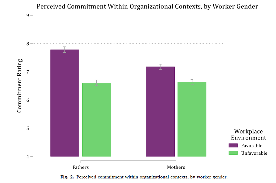
Although we find evidence that particular aspects of organizational policy and workplace culture about paid parental leave influence perceptions of worker commitment, it is important to recognize that organizational cultures are not a product of a single policy. Instead, an organizational culture reflects multiple policies and multiple aspects of workers’ attitudes and behaviors.
To illustrate the impact of organizational culture in a holistic way, we estimate predicted values of perceived commitment based on two ideal types of organizational culture: (1) favorable workplace environment and (2) unfavorable workplace environment (Long and Freese, 2014; Mize, 2019).
We define a favorable workplace environment as +1 SD weeks of leave offered and +1 SD wage replacement for mothers, and +1 SD weeks of leave offered, +1 SD wage replacement, a supportive workplace culture, and a “paternity” leave policy for fathers … In contrast, we define an unfavorable workplace environment as…