7.1 Interaction Effects (AKA Moderation)

  • Race-ethnicity
  • Gender
  • Social class
    • Educational attainment
    • Occupations
    • Income
  • Politics
    • Party affiliation
    • Beliefs
    • Behavior
  • Age
    • Cohorts
    • Life stages
    • Periods
  • Sexuality
  • Religion
    • Affiliation
    • Beliefs
    • Behavior
  • Space / geography
    • Countries
    • States
    • Cultures (and subcultures)
    • Rural vs suburban vs urban
    • Neighborhoods
    • Schools
  • Family structures

Intersecting effects

  • Often, we think an effect may operate differently across contexts or groups
    • Will a new medical treatment be equally effective across all ages?
    • Does aging result in declining physical health at the same rate for all racial-ethnic groups?
    • Are Democrats and Republicans similarly persuaded by a campaign ad?
    • Etc.
  • Intersectionality makes this argument explicit (Hill Collins and Bilge 2020)
    • E.g., The experience of being a black woman ≠ black + woman
      • The intersection produces a unique experience and effect*

*See some recent empirical evidence on this in Heiserman 2023 and Mize 2025

Interaction effects in linear regression

“Interaction effects exist when the effect of one independent variable is contingent on the level of another independent variable.” (Mize 2019 p.81)

  • In a linear regression model with no nonlinearities, consider what an interaction (product) term allows in the predictions (here with one continuous IV and one binary IV)

\[\widehat{y} = \beta_{0} + \beta_{c}c_{i} + \beta_{b}b_{i} + \beta_{cXb}{cXb}_{i} + \ldots\]

\[\widehat{{wages}_{i}} = \beta_{0} + \beta_{age}{age}_{i} + \beta_{woman}{woman}_{i} + \beta_{ageXwoman}{ageXwoman}_{i} + \ldots\]

\[\widehat{{wages}_{i}} = 4.09 + 0.26{age}_{i} + 0.00{woman}_{i} - 0.13{ageXwoman}_{i} + \ldots\]

  • What does the coefficient on the interaction (product) term represent?
    • Do men and women receive the same returns for aging?
use "https://tdmize.github.io/data/data/cda_gss", clear
(cda_gss.dta |  GSS 1972-2021 CDA - Categorical Data Analysis | date created 202
> 3)
*7.1.a & 7.1.b - linear model interaction ex: continuous X binary
qui regress wages i.woman c.age i.college i.race3 i.married i.parent ///
    if employed == 1
qui margins, at(age=(18(5)83) woman=(0 1))
marginsplot, noci ytitle("Predicted Hourly Wages") xtitle("Age in Years") ///
    title("[7.1.a] Predicted Hourly Wages Based on Age and Gender", size(mediu
m)) ///
    subtitle("Intercept Shift - No Interaction Term") ylabel(0(5)30) ///
    xlabel(20(10)80) legend(position(6)) saving(noint, replace)
Variables that uniquely identify margins: age woman
file noint.gph saved
qui regress wages i.woman##c.age i.college i.race3 i.married i.parent ///
    if employed == 1
qui margins, at(age=(18(5)83) woman=(0 1))
marginsplot, noci ytitle("Predicted Hourly Wages") xtitle("Age in Years") ///
    title("[7.1.b] Predicted Hourly Wages Based on Age and Gender", size(mediu
m)) ///
    subtitle("Interaction Term: Age X Gender") ylabel(0(5)30) ///
    xlabel(20(10)80) legend(position(6)) saving(intterm, replace)
Variables that uniquely identify margins: age woman
file intterm.gph saved
graph combine noint.gph intterm.gph

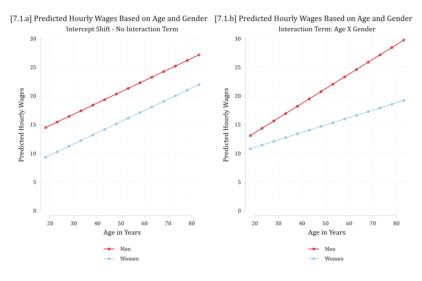
[7.1.a and 7.1.b] Two panels of predicted hourly wages by age (18 to 83) for men and women. Left, with no interaction term: two parallel rising lines, men above women by the same amount at every age. Right, with an age by gender interaction term: men's line rises more steeply than women's, so the gender gap widens with age.

library(haven)           # import Stata data and labels
library(dplyr)           # data manipulation
library(ggplot2)         # graphs
library(marginaleffects) # predictions and marginal effects
library(cleanplots)      # graph scheme
cleanplots_defaults()

gss <- read_dta("https://tdmize.github.io/data/data/cda_gss.dta")

# Keep model variables for the employed; drop any missing data
emp <- gss |>
  filter(employed == 1) |>
  select(wages, woman, age, college, race3, married, parent)
emp <- emp[complete.cases(emp), ] |>
  mutate(across(c(woman, college, race3, married, parent), as_factor))

# 7.1.a & 7.1.b - linear model interaction ex: continuous X binary
noint <- lm(wages ~ woman + age + college + race3 + married + parent, data = emp)
intterm <- lm(wages ~ woman * age + college + race3 + married + parent, data = emp)

grid <- datagrid(model = noint, age = seq(18, 83, 5), woman = unique,
  grid_type = "counterfactual")
pr <- bind_rows(
  "[7.1.a] Intercept Shift - No Interaction Term" =
    avg_predictions(noint, by = c("age", "woman"), newdata = grid),
  "[7.1.b] Interaction Term: Age X Gender" =
    avg_predictions(intterm, by = c("age", "woman"), newdata = grid),
  .id = "model")

ggplot(pr, aes(x = age, y = estimate, color = woman)) +
  geom_line() +
  geom_point() +
  facet_wrap(~ model, labeller = label_wrap_gen(35)) +
  scale_x_continuous(breaks = seq(20, 80, 10)) +
  scale_y_continuous(breaks = seq(0, 30, 5), limits = c(0, 30)) +
  labs(title = "Predicted Hourly Wages Based on Age and Gender",
    x = "Age in Years", y = "Predicted Hourly Wages", color = NULL)

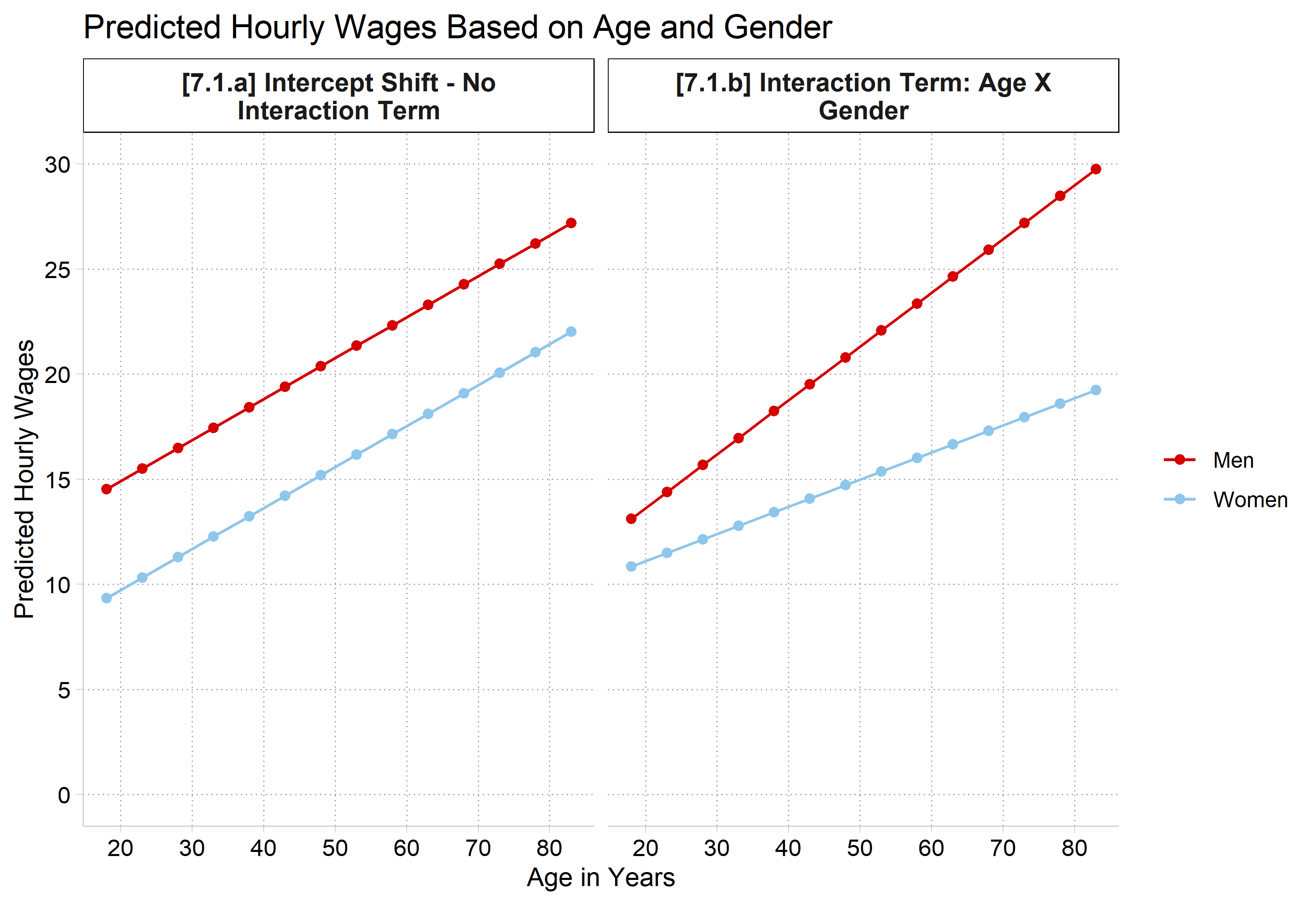
[7.1.a and 7.1.b] Two panels of predicted hourly wages by age (18 to 83) for men and women. Left, with no interaction term: two parallel rising lines, men above women by the same amount at every age. Right, with an age by gender interaction term: men's line rises more steeply than women's, so the gender gap widens with age.

Ex interaction effect with nominal IVs

  • What about when we have only nominal IVs in the interaction?
    • Consider what an interaction (product) term allows in the predictions (using two binary IVs for simplicity)

\[\widehat{y} = \beta_{0} + \beta_{b1}{b1}_{i} + \beta_{b2}{b2}_{i} + \beta_{b1Xb2}{b1Xb2}_{i} + \ldots\]

\[\widehat{{wages}_{i}} = \beta_{0} + \beta_{woman}{woman}_{i} + \beta_{college}{college}_{i} + \beta_{womanXcollege}{womanXcollege}_{i} + \ldots\]

\[\widehat{{wages}_{i}} = 6.36 - 4.72{woman}_{i} + 10.47{college}_{i} - 1.56{womanXcollege}_{i} + \ldots\]

  • What does the coefficient on the interaction (product) term represent?
    • Is college the great equalizer? Does it reduce the gender gap?
*7.1.c & 7.1.d - linear model interaction ex: binary X binary
qui regress wages i.woman i.college c.age i.race4 i.married i.parent
est store no_int
qui margins college, at(woman=0) post
est store pr_men
est restore no_int
(results no_int are active now)
qui margins college, at(woman=1) post
est store pr_wom
coefplot pr_men pr_wom, ///
    recast(bar) vertical barw(0.3) citop ///
    ylab(0(5)35) legend(order(1 "Men" 3 "Women") pos(6) row(1)) ///
    ytitle("Hourly wages") ///
    xtitle("Educational attainment") ///
    title("[7.1.c] Hourly wages by gender and education") ///
    subtitle("No interaction term") saving(bin_no, replace)
file bin_no.gph saved
*add an interaction
qui regress wages i.woman##i.college c.age i.race4 i.married i.parent
est store w_int
qui margins college, at(woman=0) post
est store pr_men
est restore w_int
(results w_int are active now)
qui margins college, at(woman=1) post
est store pr_wom
coefplot pr_men pr_wom, ///
    recast(bar) vertical barw(0.3) citop ///
    ylab(0(5)35) legend(order(1 "Men" 3 "Women") pos(6) row(1)) ///
    ytitle("Hourly wages") ///
    xtitle("Educational attainment") ///
    title("[7.1.d] Hourly wages by gender and education") ///
    subtitle("Including gender X college interaction") saving(bin_int, replace
)
file bin_int.gph saved
graph combine bin_no.gph bin_int.gph

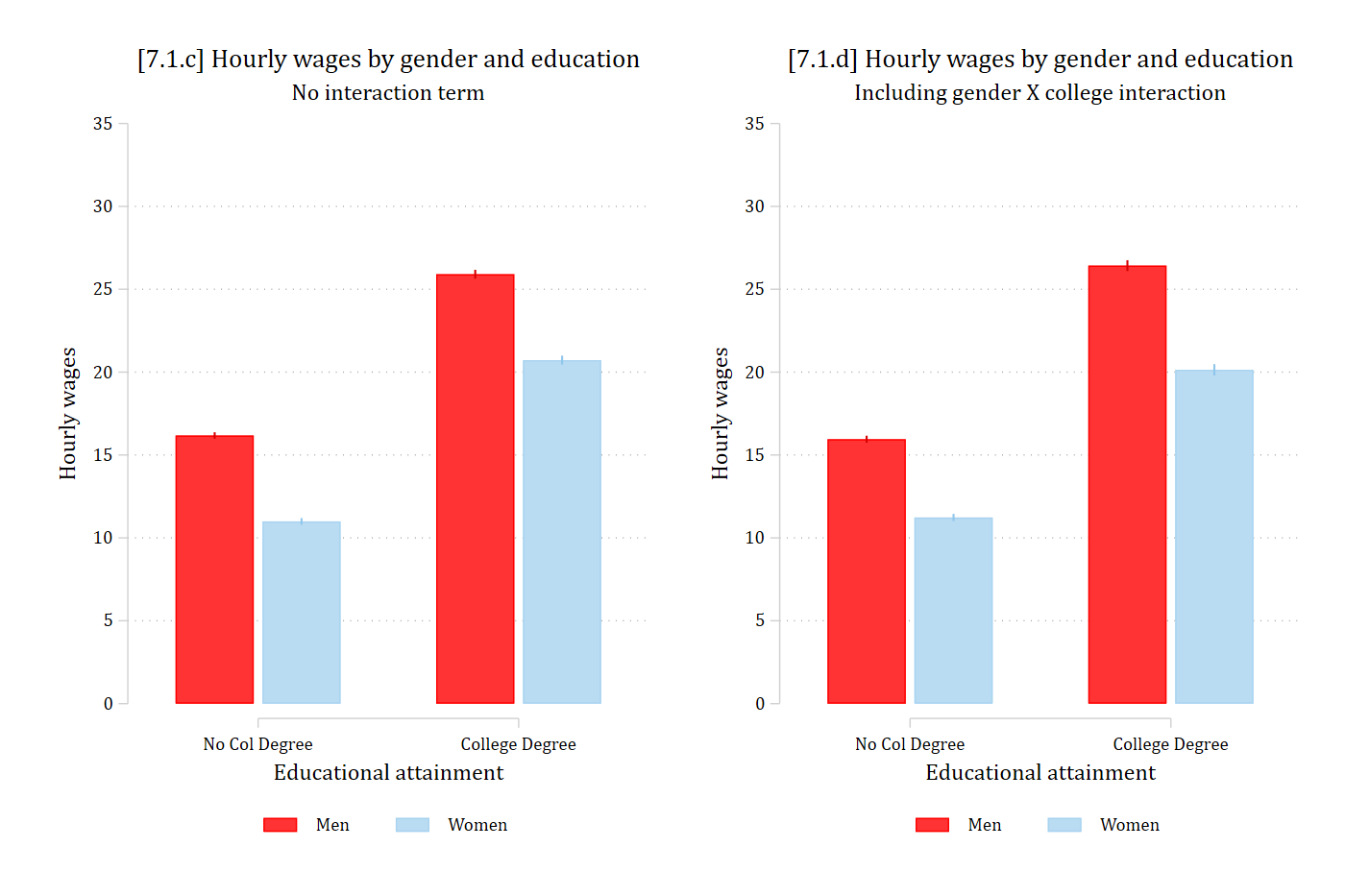
[7.1.c and 7.1.d] Two bar charts of predicted hourly wages by college degree for men and women. Left, with no interaction term: about $16 for men and $11 for women without a degree, and about $26 for men and $21 for women with a degree, the same gap at both levels. Right, with a gender by college interaction: about $16 and $11 without a degree, and about $26.5 and $20 with a degree, a wider gender gap among college graduates.

# Keep model variables; drop any missing data
wg <- gss |>
  select(wages, woman, college, age, race4, married, parent)
wg <- wg[complete.cases(wg), ] |>
  mutate(across(c(woman, college, race4, married, parent), as_factor))

# 7.1.c & 7.1.d - linear model interaction ex: binary X binary
no_int <- lm(wages ~ woman + college + age + race4 + married + parent, data = wg)
w_int <- lm(wages ~ woman * college + age + race4 + married + parent, data = wg)

grid <- datagrid(model = no_int, college = unique, woman = unique,
  grid_type = "counterfactual")
pr <- bind_rows(
  "[7.1.c] No interaction term" =
    avg_predictions(no_int, by = c("college", "woman"), newdata = grid),
  "[7.1.d] Including gender X college interaction" =
    avg_predictions(w_int, by = c("college", "woman"), newdata = grid),
  .id = "model")

ggplot(pr, aes(x = college, y = estimate, fill = woman)) +
  geom_col(position = position_dodge(.7), width = .6) +
  geom_errorbar(aes(ymin = conf.low, ymax = conf.high),
    position = position_dodge(.7), width = .1) +
  facet_wrap(~ model, labeller = label_wrap_gen(35)) +
  scale_y_continuous(breaks = seq(0, 35, 5), limits = c(0, 35)) +
  labs(title = "Hourly wages by gender and education",
    x = "Educational attainment", y = "Hourly wages", fill = NULL)

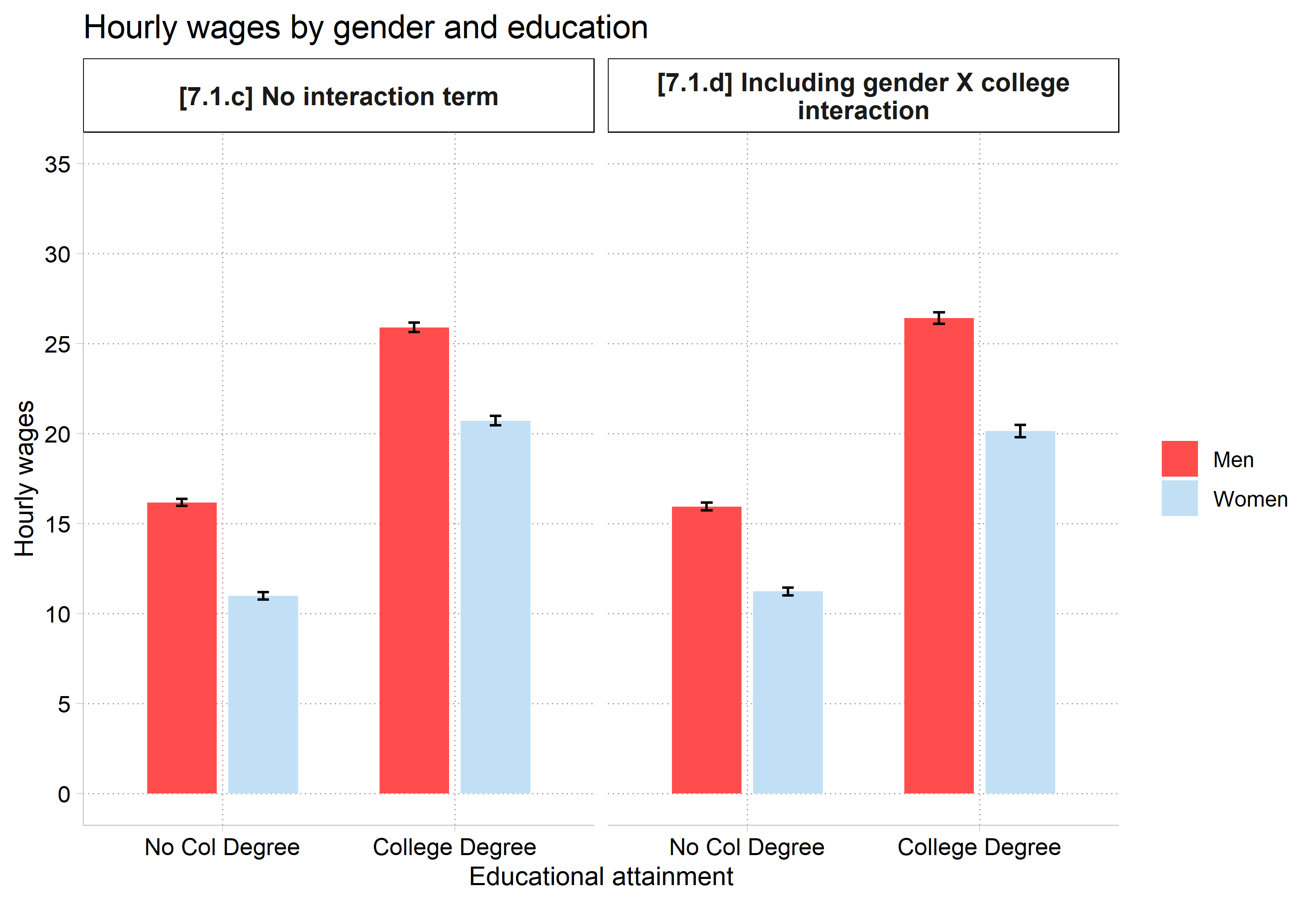
[7.1.c and 7.1.d] Two bar charts of predicted hourly wages by college degree for men and women. Left, with no interaction term: about $16 for men and $11 for women without a degree, and about $26 for men and $21 for women with a degree, the same gap at both levels. Right, with a gender by college interaction: about $16 and $11 without a degree, and about $26.5 and $20 with a degree, a wider gender gap among college graduates.

*For details on gender inequality for highly educated workers see Quadlin et al. 2023

Nonlinear interaction effects

  • For any nonlinear model, the coefficient on the interaction term is not a test of interaction (e.g., logit and probit). Why?
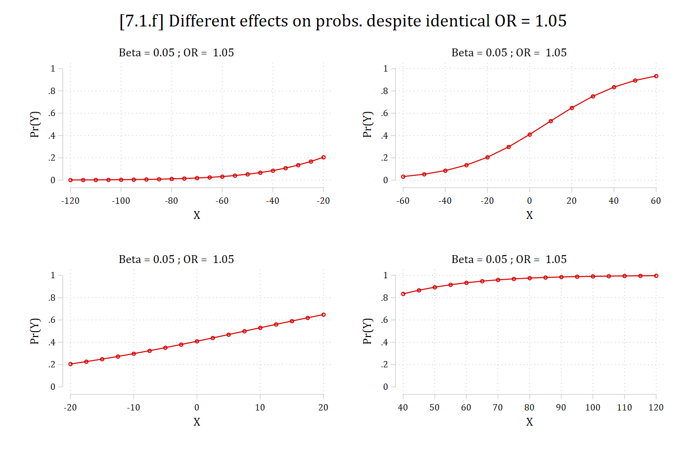
  • Consider the variation in possible relationships observed in your data from a single parameter estimate (β = 0.05 for a continuous IV)
// Exs of possible effects in predictions given same beta //
use "https://tdmize.github.io/data/data/scireview3", clear
(Biochemist data - updated for CDA Stata guide)
*7.1.e - full logit curve; OR = 1.05
qui logit faculty i.fellow c.totpub c.phd
qui margins, at(totpub=(-120(10)120))
marginsplot, noci ylabel(0(0.2)1) xlabel(-120(20)120) ///
    xtitle("X") ytitle("Pr(Y)") title("[7.1.e] Beta = 0.05 ; OR =  1.05")
Variables that uniquely identify margins: totpub

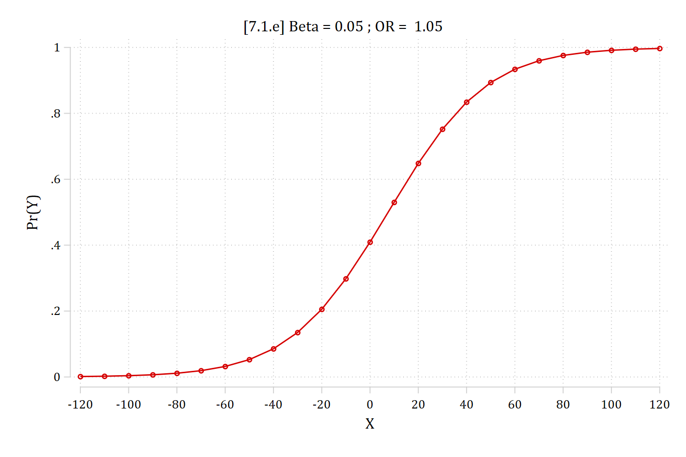
[7.1.e] The full S-shaped logit curve of Pr(Y) for X from -120 to 120 with beta = 0.05: near 0 below X = -60, rising steeply through about 0.4 at X = 0, and leveling off near 1 above X = 60.

# Exs of possible effects in predictions given same beta
sci <- read_dta("https://tdmize.github.io/data/data/scireview3.dta") |>
  mutate(fellow = as_factor(fellow))

# 7.1.e - full logit curve; OR = 1.05
scimod <- glm(faculty ~ fellow + totpub + phd, data = sci,
  family = binomial(link = "logit"))

pr_x <- function(xvals) {
  avg_predictions(scimod, by = "totpub",
    newdata = datagrid(totpub = xvals, grid_type = "counterfactual"))
}

ggplot(pr_x(seq(-120, 120, 10)), aes(x = totpub, y = estimate)) +
  geom_line(color = "red") +
  geom_point(color = "red") +
  scale_x_continuous(breaks = seq(-120, 120, 20)) +
  scale_y_continuous(breaks = seq(0, 1, .2), limits = c(0, 1)) +
  labs(title = "[7.1.e] Beta = 0.05 ; OR =  1.05", x = "X", y = "Pr(Y)")

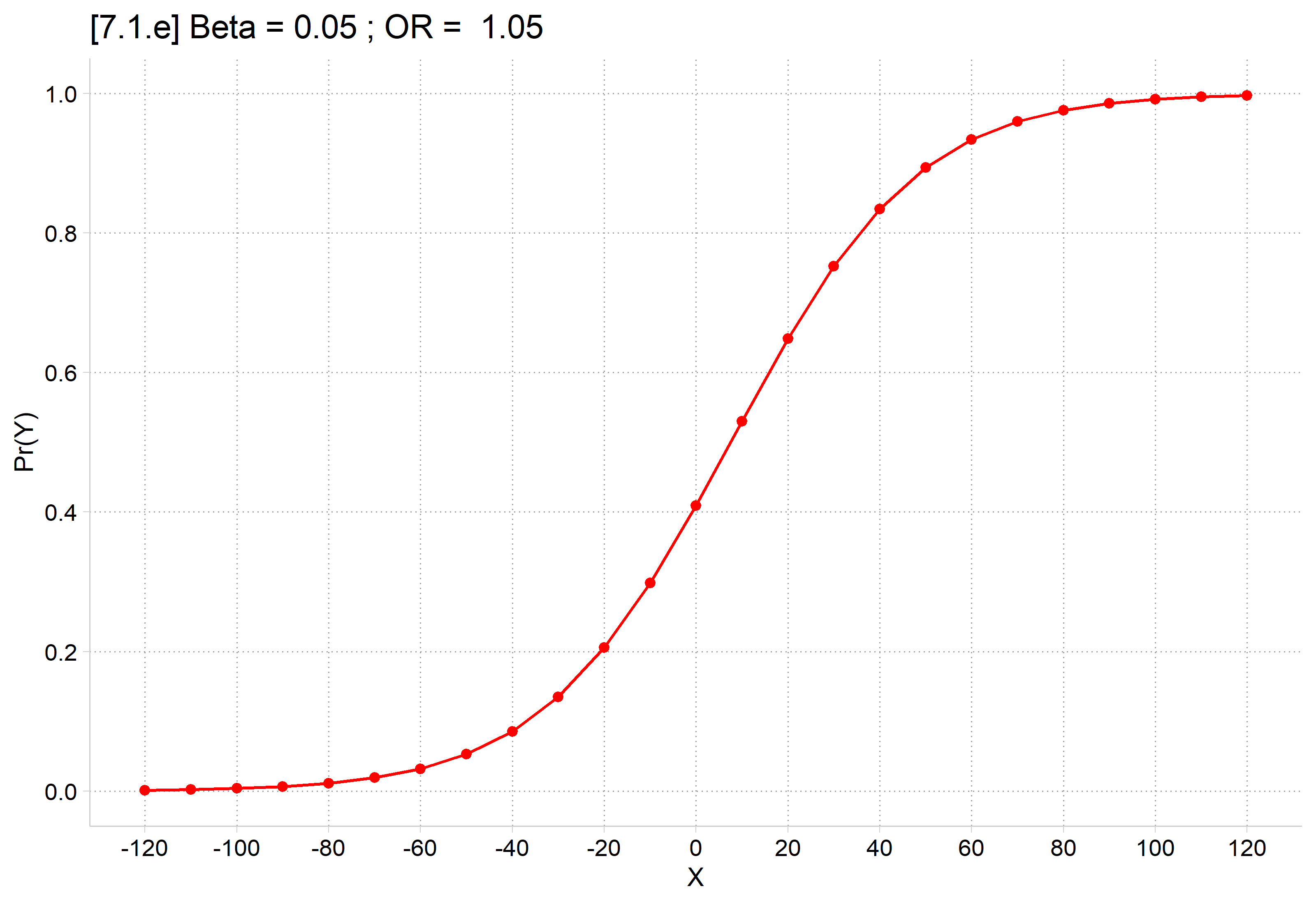
[7.1.e] The full S-shaped logit curve of Pr(Y) for X from -120 to 120 with beta = 0.05: near 0 below X = -60, rising steeply through about 0.4 at X = 0, and leveling off near 1 above X = 60.

qui margins, at(totpub=(-120(5)-20))
marginsplot, noci ylabel(0(0.2)1) xlabel(-120(20)-20) xtitle("X")  ///
    ytitle("Pr(Y)") title("Beta = 0.05 ; OR =  1.05") name(ex1, replace)
Variables that uniquely identify margins: totpub
qui margins, at(totpub=(-60(10)60))
marginsplot, noci ylabel(0(0.2)1) xlabel(-60(20)60) xtitle("X") ///
    ytitle("Pr(Y)") title("Beta = 0.05 ; OR =  1.05") name(ex2, replace)
Variables that uniquely identify margins: totpub
qui margins, at(totpub=(-20(2.5)20))
marginsplot, noci ylabel(0(0.2)1) xlabel(-20(10)20) xtitle("X") ///
    ytitle("Pr(Y)") title("Beta = 0.05 ; OR =  1.05") name(ex3, replace)
Variables that uniquely identify margins: totpub
qui margins, at(totpub=(40(5)120))
marginsplot, noci ylabel(0(0.2)1) xlabel(40(10)120) xtitle("X") ///
    ytitle("Pr(Y)") title("Beta = 0.05 ; OR =  1.05") name(ex4, replace)
Variables that uniquely identify margins: totpub
*7.1.f
graph combine ex1 ex2 ex3 ex4, ///
    title("[7.1.f] Different effects on probs. despite identical OR = 1.05")

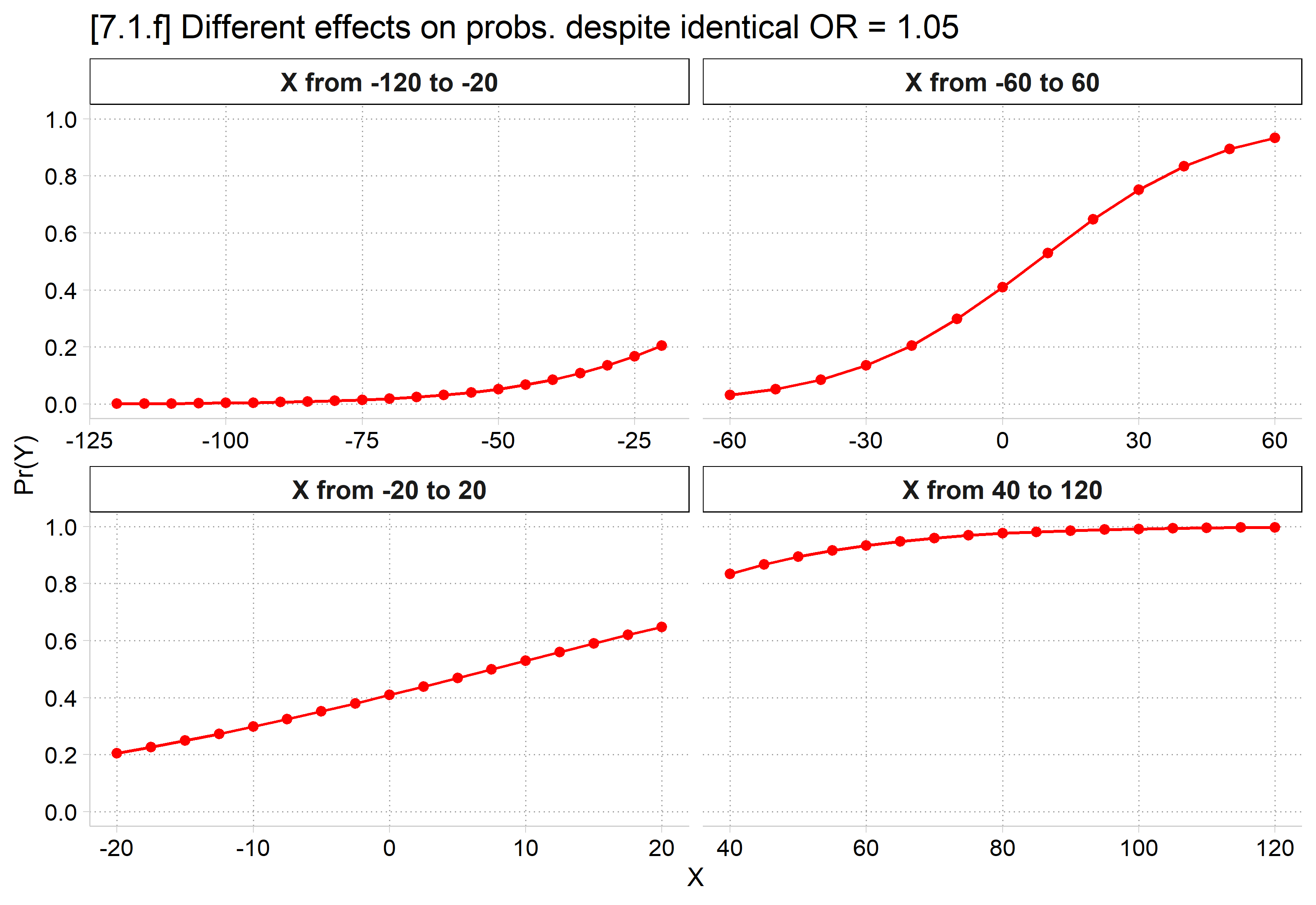
[7.1.f] Four panels showing parts of the same logit curve (beta = 0.05) over different ranges of X: from -120 to -20 the probability barely rises from 0 to about 0.2; from -60 to 60 it rises steeply in an S shape from about 0.03 to 0.93; from -20 to 20 it rises almost linearly from about 0.2 to 0.65; from 40 to 120 it is nearly flat, from about 0.84 to 1.

# 7.1.f - the same curve over four ranges of X
pr4 <- bind_rows(
  "X from -120 to -20" = pr_x(seq(-120, -20, 5)),
  "X from -60 to 60" = pr_x(seq(-60, 60, 10)),
  "X from -20 to 20" = pr_x(seq(-20, 20, 2.5)),
  "X from 40 to 120" = pr_x(seq(40, 120, 5)),
  .id = "range") |>
  mutate(range = factor(range, levels = unique(range)))

ggplot(pr4, aes(x = totpub, y = estimate)) +
  geom_line(color = "red") +
  geom_point(color = "red") +
  facet_wrap(~ range, scales = "free_x") +
  scale_y_continuous(breaks = seq(0, 1, .2), limits = c(0, 1)) +
  labs(title = "[7.1.f] Different effects on probs. despite identical OR = 1.05",
    x = "X", y = "Pr(Y)")

[7.1.f] Four panels showing parts of the same logit curve (beta = 0.05) over different ranges of X: from -120 to -20 the probability barely rises from 0 to about 0.2; from -60 to 60 it rises steeply in an S shape from about 0.03 to 0.93; from -20 to 20 it rises almost linearly from about 0.2 to 0.65; from 40 to 120 it is nearly flat, from about 0.84 to 1.

Inherently interactive nature of logit/probit models

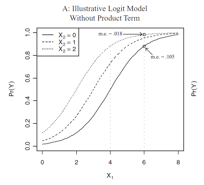
Panel A from Berry, DeMeritt, and Esarey (2010), an illustrative logit model without a product term: three S-shaped curves of Pr(Y) against X1 for X2 = 0, 1, and 2, shifted left as X2 increases. The marginal effect of X1 at X1 = 6 is .105 on one curve but only .018 on another.

Figure from Berry, DeMeritt, and Esarey 2010 AJPS

  • In the example above with one continuous IV and one nominal IV, the logit/probit model is interactive because of intercept shifts produced by the nominal IV
    • That is, the β coefficient (which determines the slope) is invariant across the levels of the nominal IV
    • The effect on the probabilities is not constant due to the intercept shift
      • This is because of “compression”—i.e. that the predicted probability curve flattens at Pr(y) = 0 and Pr(y) = 1—thus all three of the curves above converge/compress to have the same slope at both extremes
  • Consider the following example with real data (Add Health Wave 4)
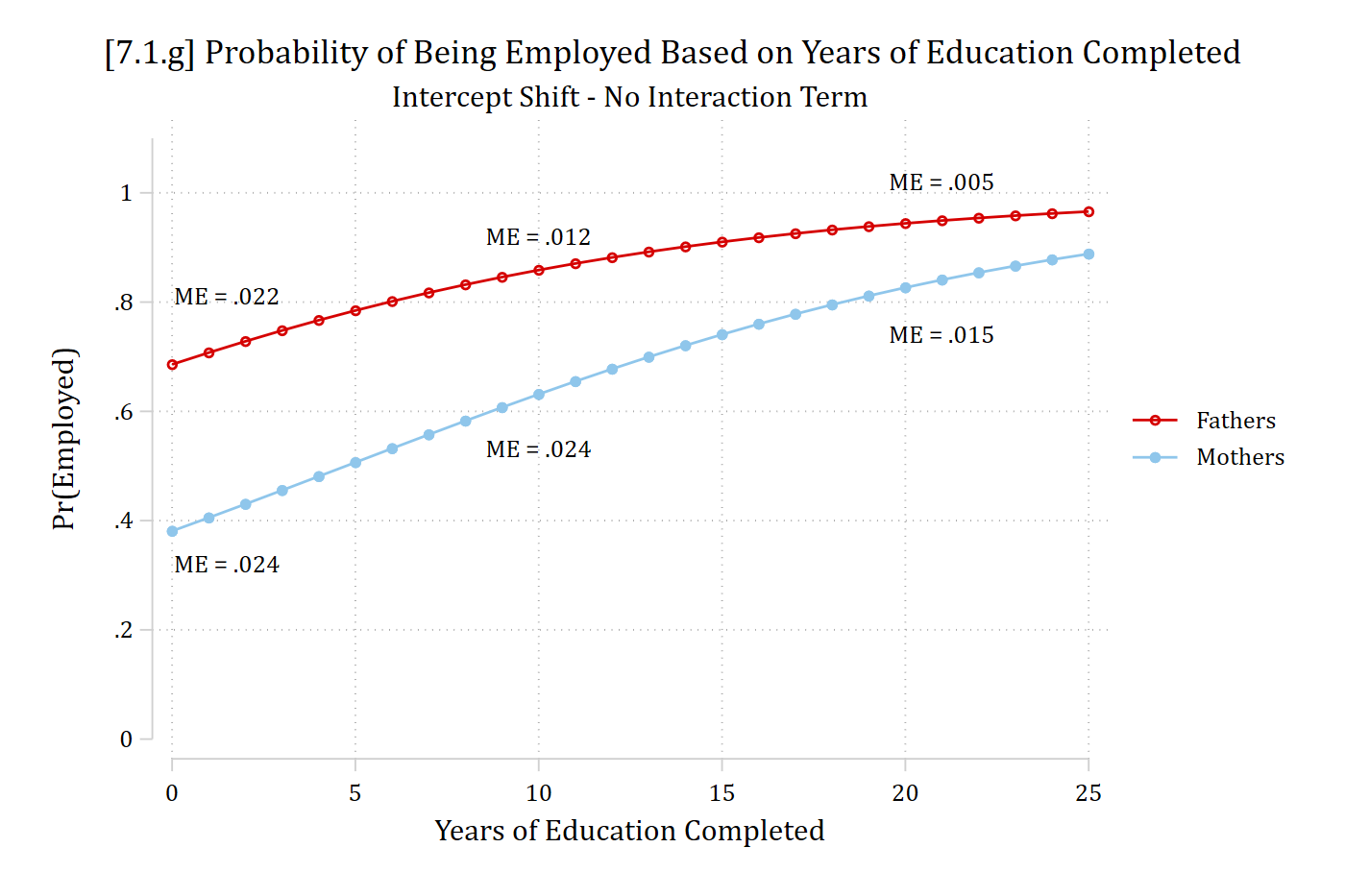
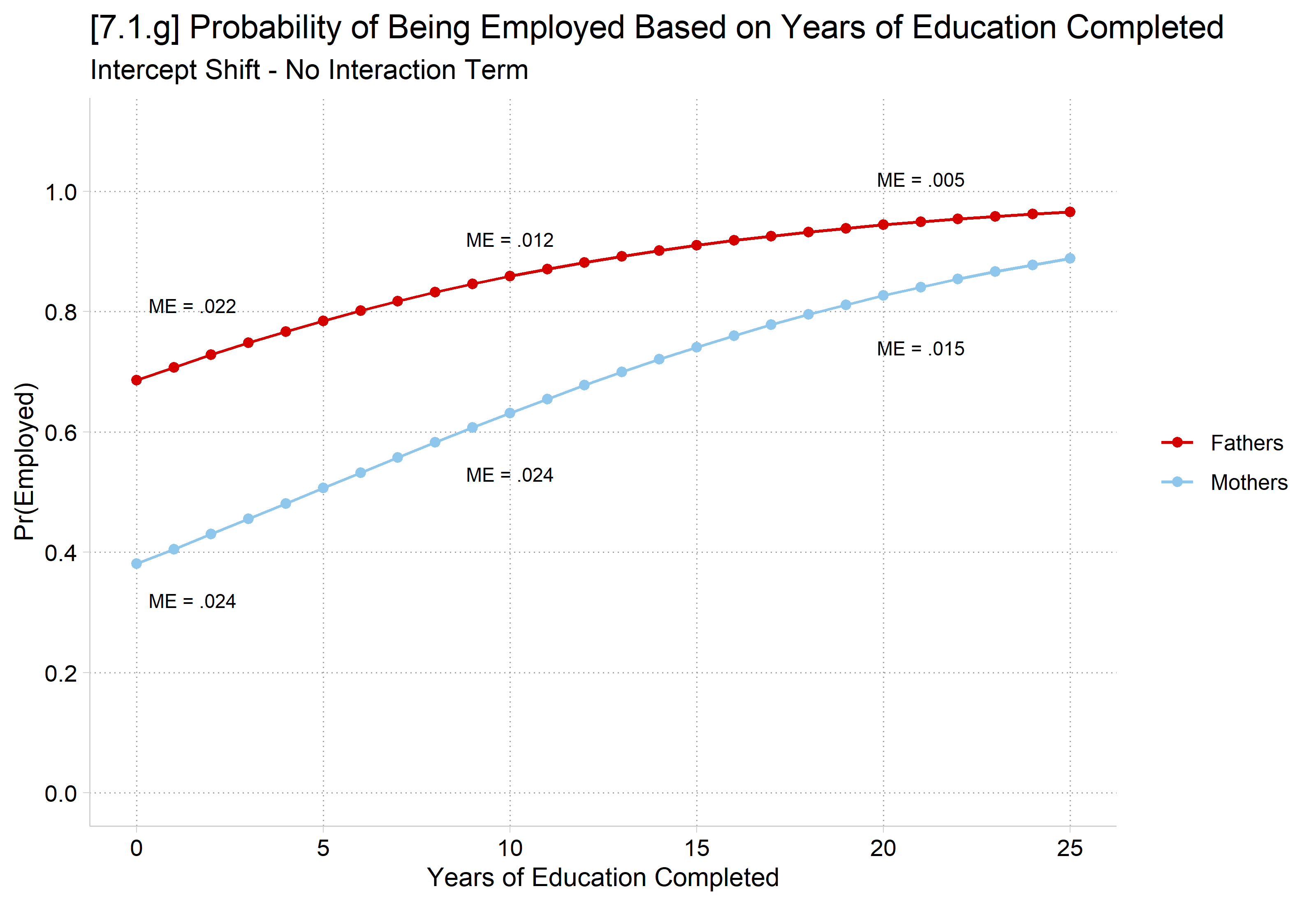
    • Pr(Employed) for mothers and fathers, based on years of education completed
// Logit Examples w/ and w/o interaction terms //
use "https://tdmize.github.io/data/data/addhealth4", clear
(addhealth4_dmv.dta | Add Health Wave IV | DMV Workshop)
*Intercept Shift in Logit
qui logit employed c.edyrs i.woman if parrole == 1, or nolog
est store intshift
*7.1.g - Estimate MEs at various places in data
mtable, dydx(edyrs) at(woman=(0 1) edyrs=(0 10 20 25))
Expression: Pr(employed), predict()

           |    edyrs     woman   d Pr(y)
 ----------+-----------------------------
         1 |        0         0     0.022
         2 |        0         1     0.024
         3 |       10         0     0.012
         4 |       10         1     0.024
         5 |       20         0     0.005
         6 |       20         1     0.015
         7 |       25         0     0.003
         8 |       25         1     0.010

Specified values where .n indicates no values specified with at()

           |  No at()
 ----------+---------
   Current |       .n
qui margins, at(edyrs=(0(1)25) woman=(0 1))
marginsplot, noci legend(order(1 "Fathers" 2 "Mothers")) ///
    ytitle("Pr(Employed)") xtitle("Years of Education Completed") ///
    title("[7.1.g] Probability of Being Employed Based on Years of Education C
ompleted", size(medium)) ///
    subtitle("Intercept Shift - No Interaction Term") ylabel(0(0.2)1.1) xlabel
(0(5)25) ///
    text(.32 1.5 "ME = .024" .81 1.5 "ME = .022" ///
        .53 10 "ME = .024" .92 10 "ME = .012" ///
        .74 21 "ME = .015" 1.02 21 "ME = .005", size(small))
Variables that uniquely identify margins: edyrs woman

[7.1.g] Predicted probability of being employed by years of education (0 to 25) for fathers and mothers, from a logit model with no interaction term. Fathers' probability rises from about 0.69 to 0.96 and mothers' from about 0.38 to 0.89. The marginal effect of education is about .022 for fathers and .024 for mothers at 0 years, .012 and .024 at 10 years, and .005 and .015 at 20 to 25 years: the curves converge as both approach 1.

# Logit Examples w/ and w/o interaction terms
ah4 <- read_dta("https://tdmize.github.io/data/data/addhealth4.dta") |>
  filter(parrole == 1) |>
  mutate(woman = factor(woman, levels = 0:1, labels = c("Fathers", "Mothers")))

# Intercept Shift in Logit
intshift <- glm(employed ~ edyrs + woman, data = ah4,
  family = binomial(link = "logit"))

# 7.1.g - Estimate MEs at various places in data
slopes(intshift, variables = "edyrs",
  newdata = datagrid(woman = unique, edyrs = c(0, 10, 20, 25)))

   woman edyrs Estimate Std. Error     z Pr(>|z|)     S   2.5 %  97.5 %
 Fathers     0  0.02206   0.009343  2.36  0.01823   5.8 0.00375 0.04037
 Fathers    10  0.01242   0.004475  2.78  0.00551   7.5 0.00365 0.02119
 Fathers    20  0.00539   0.000864  6.24  < 0.001  31.1 0.00370 0.00709
 Fathers    25  0.00338   0.000423  8.00  < 0.001  49.5 0.00255 0.00421
 Mothers     0  0.02415   0.004463  5.41  < 0.001  23.9 0.01540 0.03289
 Mothers    10  0.02383   0.007352  3.24  0.00119   9.7 0.00942 0.03824
 Mothers    20  0.01467   0.002495  5.88  < 0.001  27.9 0.00978 0.01956
 Mothers    25  0.01015   0.000591 17.18  < 0.001 217.4 0.00900 0.01131

Term: edyrs
Type: response
Comparison: dY/dX
pr_ed <- function(model, xvals) {
  avg_predictions(model, by = c("edyrs", "woman"),
    newdata = datagrid(edyrs = xvals, woman = unique, grid_type = "counterfactual"))
}

ggplot(pr_ed(intshift, 0:25), aes(x = edyrs, y = estimate, color = woman)) +
  geom_line() +
  geom_point() +
  annotate("text", size = 3,
    x = c(1.5, 1.5, 10, 10, 21, 21), y = c(.32, .81, .53, .92, .74, 1.02),
    label = c("ME = .024", "ME = .022", "ME = .024", "ME = .012", "ME = .015",
      "ME = .005")) +
  scale_x_continuous(breaks = seq(0, 25, 5)) +
  scale_y_continuous(breaks = seq(0, 1, .2), limits = c(0, 1.1)) +
  labs(title = "[7.1.g] Probability of Being Employed Based on Years of Education Completed",
    subtitle = "Intercept Shift - No Interaction Term",
    x = "Years of Education Completed", y = "Pr(Employed)", color = NULL)

[7.1.g] Predicted probability of being employed by years of education (0 to 25) for fathers and mothers, from a logit model with no interaction term. Fathers' probability rises from about 0.69 to 0.96 and mothers' from about 0.38 to 0.89. The marginal effect of education is about .022 for fathers and .024 for mothers at 0 years, .012 and .024 at 10 years, and .005 and .015 at 20 to 25 years: the curves converge as both approach 1.

*Even though this is just part of the full logit curve, we still see interactive effects

Inherently interactive nature of logit/probit models

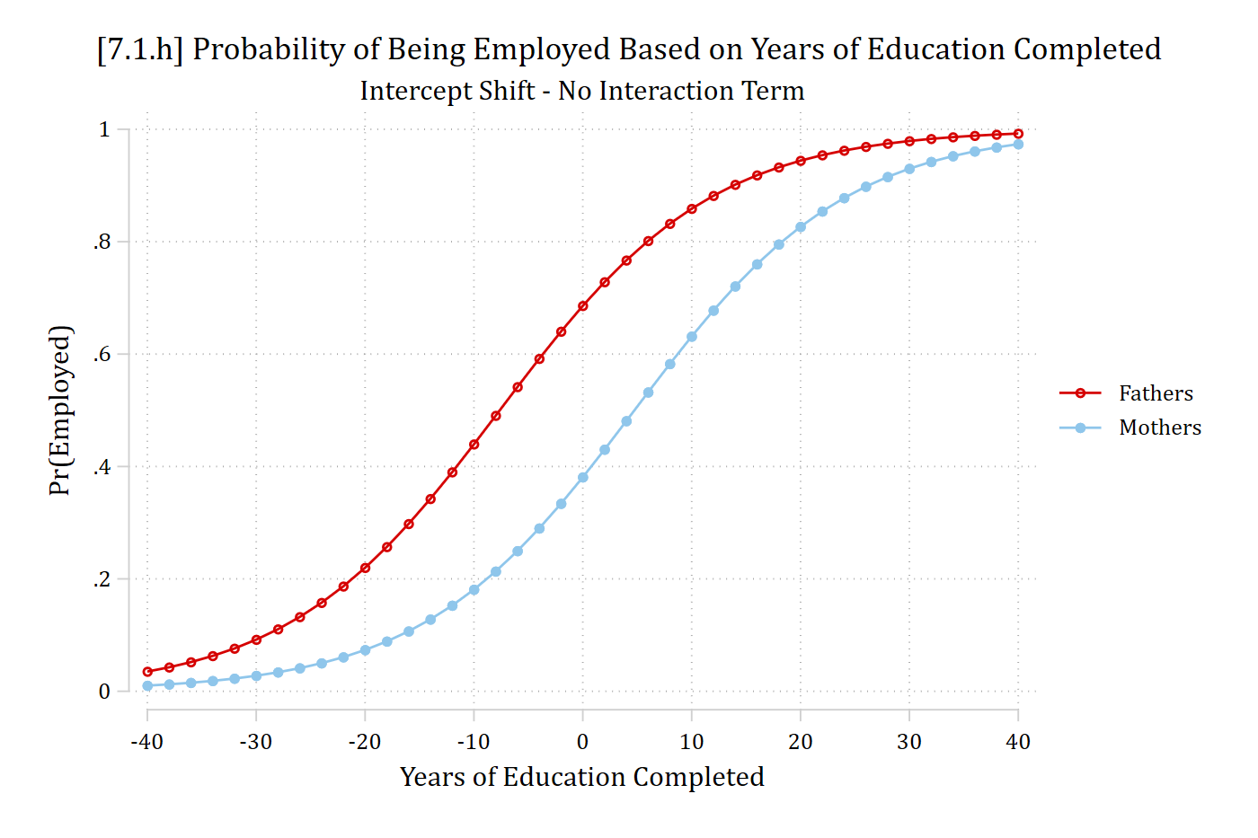
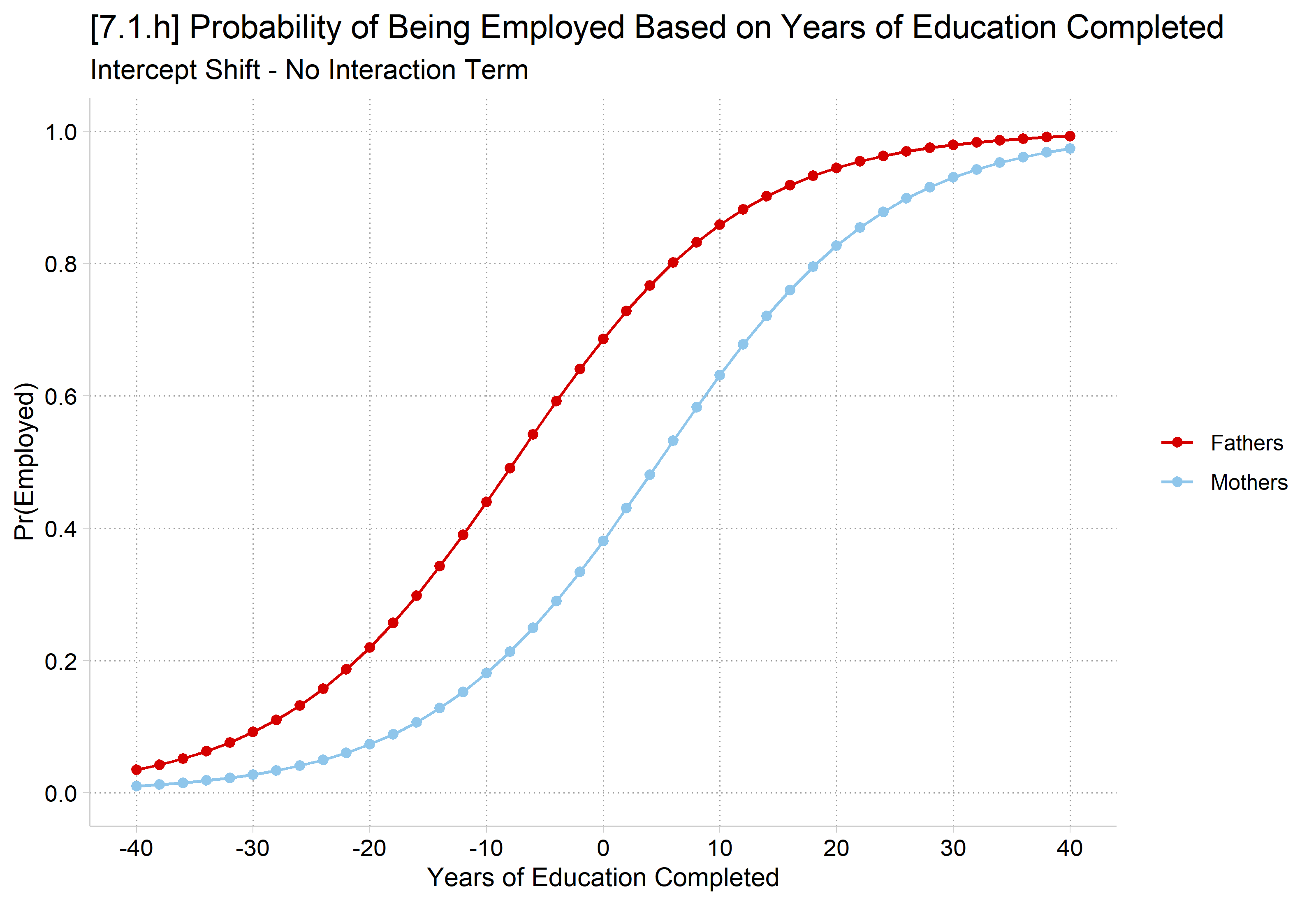
The full logit curve makes it easier to see that the overall slopes of the two curves are the same—the effects vary only because of the intercept shift

*7.1.h - Full logit curve with wider range of x
qui margins, at(edyrs=(-40(2)40) woman=(0 1))
marginsplot, noci legend(order(1 "Fathers" 2 "Mothers")) ///
    ytitle("Pr(Employed)") xtitle("Years of Education Completed") ///
    title("[7.1.h] Probability of Being Employed Based on Years of Education C
ompleted", size(medium)) ///
    subtitle("Intercept Shift - No Interaction Term") ylabel(0(0.2)1) xlabel(-
40(10)40)
Variables that uniquely identify margins: edyrs woman

[7.1.h] The full logit curves of the probability of being employed for fathers and mothers, with years of education extended from -40 to 40: two S-shaped curves with the same shape, the mothers' curve shifted to the right of the fathers' curve. Both start near 0 and end near 1.

# 7.1.h - Full logit curve with wider range of x
ggplot(pr_ed(intshift, seq(-40, 40, 2)), aes(x = edyrs, y = estimate, color = woman)) +
  geom_line() +
  geom_point() +
  scale_x_continuous(breaks = seq(-40, 40, 10)) +
  scale_y_continuous(breaks = seq(0, 1, .2), limits = c(0, 1)) +
  labs(title = "[7.1.h] Probability of Being Employed Based on Years of Education Completed",
    subtitle = "Intercept Shift - No Interaction Term",
    x = "Years of Education Completed", y = "Pr(Employed)", color = NULL)

[7.1.h] The full logit curves of the probability of being employed for fathers and mothers, with years of education extended from -40 to 40: two S-shaped curves with the same shape, the mothers' curve shifted to the right of the fathers' curve. Both start near 0 and end near 1.

The effect of interaction terms in logit/probit

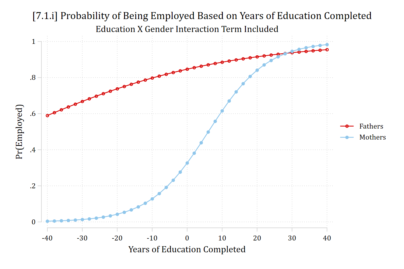
Consider the effect on the full logit curve of including an interaction (product) term

*Add interaction/product term in logit
qui logit employed c.edyrs##i.woman if parrole == 1, or nolog
est store interact
*7.1.i - Full logit curve
qui margins, at(edyrs=(-40(2)40) woman=(0 1))
marginsplot, noci legend(order(1 "Fathers" 2 "Mothers")) ///
    ytitle("Pr(Employed)") xtitle("Years of Education Completed") ///
    title("[7.1.i] Probability of Being Employed Based on Years of Education C
ompleted", size(medium)) ///
    subtitle("Education X Gender Interaction Term Included") ///
    ylabel(0(0.2)1) xlabel(-40(10)40)
Variables that uniquely identify margins: edyrs woman

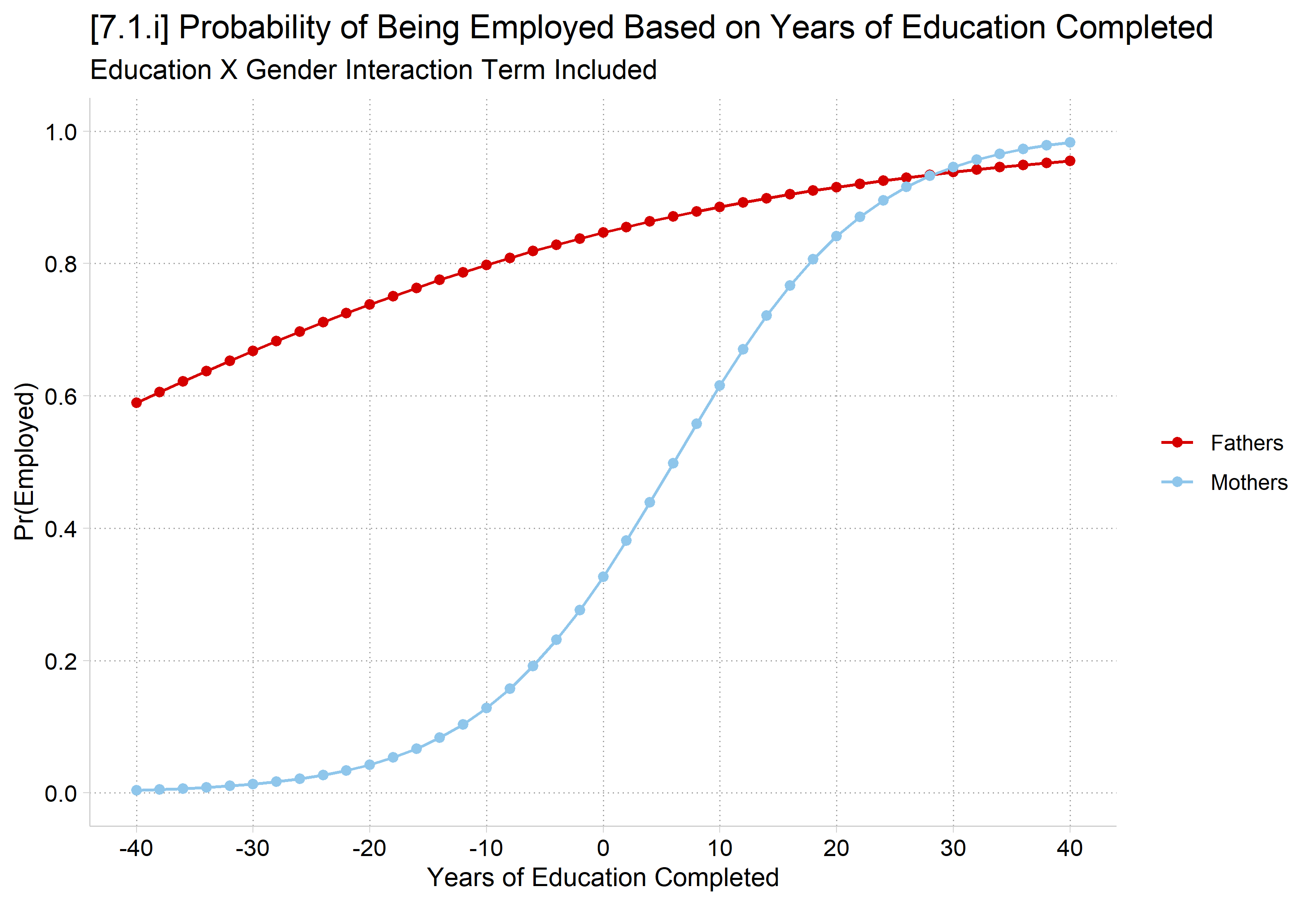
[7.1.i] Full logit curves of the probability of being employed for fathers and mothers, years of education from -40 to 40, with an education by gender interaction term: the fathers' curve is much flatter, rising slowly from about 0.6 to 0.95, while the mothers' curve is a steep S from near 0 to about 0.98, crossing the fathers' curve near 25 years.

# Add interaction/product term in logit
interact <- glm(employed ~ edyrs * woman, data = ah4, family = binomial(link = "logit"))

# 7.1.i - Full logit curve
ggplot(pr_ed(interact, seq(-40, 40, 2)), aes(x = edyrs, y = estimate, color = woman)) +
  geom_line() +
  geom_point() +
  scale_x_continuous(breaks = seq(-40, 40, 10)) +
  scale_y_continuous(breaks = seq(0, 1, .2), limits = c(0, 1)) +
  labs(title = "[7.1.i] Probability of Being Employed Based on Years of Education Completed",
    subtitle = "Education X Gender Interaction Term Included",
    x = "Years of Education Completed", y = "Pr(Employed)", color = NULL)

[7.1.i] Full logit curves of the probability of being employed for fathers and mothers, years of education from -40 to 40, with an education by gender interaction term: the fathers' curve is much flatter, rising slowly from about 0.6 to 0.95, while the mothers' curve is a steep S from near 0 to about 0.98, crossing the fathers' curve near 25 years.

*7.1.j - Estimate MEs at various places in data
mtable, dydx(edyrs) at(woman=(0 1) edyrs=(0 10 20 25))
Expression: Pr(employed), predict()

           |    edyrs     woman   d Pr(y)
 ----------+-----------------------------
         1 |        0         0     0.004
         2 |        0         1     0.026
         3 |       10         0     0.003
         4 |       10         1     0.028
         5 |       20         0     0.003
         6 |       20         1     0.016
         7 |       25         0     0.002
         8 |       25         1     0.010

Specified values where .n indicates no values specified with at()

           |  No at()
 ----------+---------
   Current |       .n
qui margins, at(edyrs=(0(1)25) woman=(0 1))
marginsplot, noci legend(order(1 "Fathers" 2 "Mothers")) ///
    ytitle("Pr(Employed)") xtitle("Years of Education Completed") ///
    title("[7.1.j] Probability of Being Employed Based on Years of Education C
ompleted", size(medium)) ///
    subtitle("Education X Gender Interaction Term Included") ylabel(0(0.2)1.1)
 xlabel(0(5)25) ///
    text(.29 1.5 "ME = .026" .92 1.5 "ME = .004" ///
        .51 10 "ME = .028" .95 10 "ME = .003" ///
        .79 21 "ME = .016" .98 21 "ME = .003", size(small))
Variables that uniquely identify margins: edyrs woman

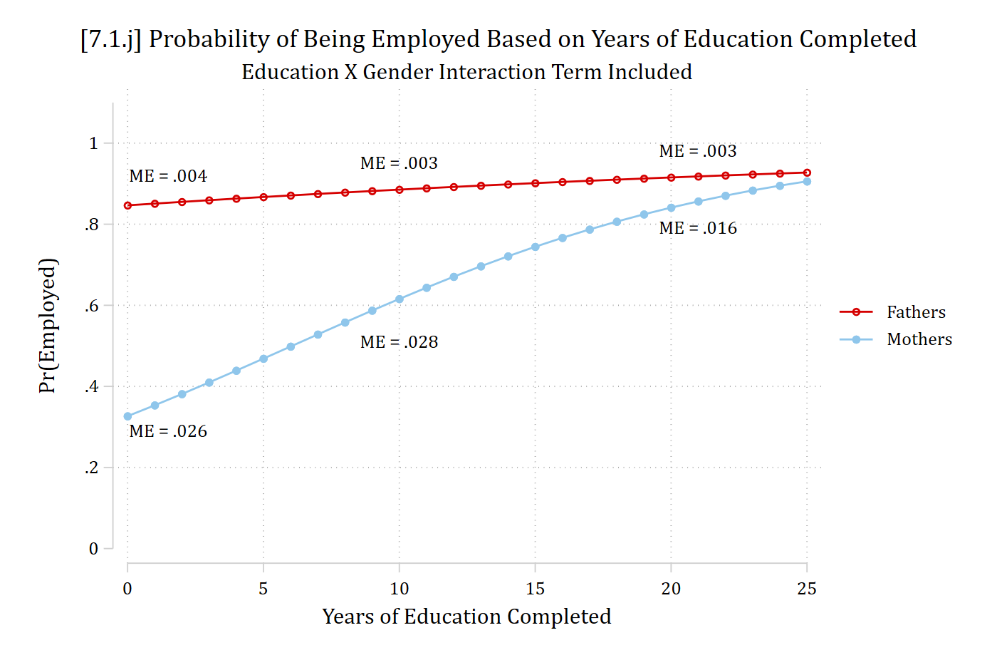
[7.1.j] Predicted probability of being employed by years of education (0 to 25) for fathers and mothers, with an education by gender interaction term. Fathers' probability is nearly flat, from about 0.85 to 0.93 (marginal effects of .004 and .003); mothers' probability rises from about 0.33 to 0.91 (marginal effects of .026 at 0 years, .028 at 10 years, and .016 at 20 years).

# 7.1.j - Estimate MEs at various places in data
slopes(interact, variables = "edyrs",
  newdata = datagrid(woman = unique, edyrs = c(0, 10, 20, 25)))

   woman edyrs Estimate Std. Error      z Pr(>|z|)     S    2.5 %  97.5 %
 Fathers     0  0.00437   0.010773  0.406    0.685   0.5 -0.01675 0.02548
 Fathers    10  0.00341   0.006990  0.488    0.625   0.7 -0.01029 0.01711
 Fathers    20  0.00261   0.004013  0.649    0.516   1.0 -0.00526 0.01047
 Fathers    25  0.00226   0.002854  0.792    0.428   1.2 -0.00333 0.00785
 Mothers     0  0.02628   0.003045  8.631   <0.001  57.2  0.02031 0.03225
 Mothers    10  0.02827   0.008397  3.367   <0.001  10.4  0.01181 0.04473
 Mothers    20  0.01597   0.002247  7.105   <0.001  39.6  0.01156 0.02037
 Mothers    25  0.01019   0.000555 18.357   <0.001 247.6  0.00910 0.01128

Term: edyrs
Type: response
Comparison: dY/dX
ggplot(pr_ed(interact, 0:25), aes(x = edyrs, y = estimate, color = woman)) +
  geom_line() +
  geom_point() +
  annotate("text", size = 3,
    x = c(1.5, 1.5, 10, 10, 21, 21), y = c(.29, .92, .51, .95, .79, .98),
    label = c("ME = .026", "ME = .004", "ME = .028", "ME = .003", "ME = .016",
      "ME = .003")) +
  scale_x_continuous(breaks = seq(0, 25, 5)) +
  scale_y_continuous(breaks = seq(0, 1, .2), limits = c(0, 1.1)) +
  labs(title = "[7.1.j] Probability of Being Employed Based on Years of Education Completed",
    subtitle = "Education X Gender Interaction Term Included",
    x = "Years of Education Completed", y = "Pr(Employed)", color = NULL)

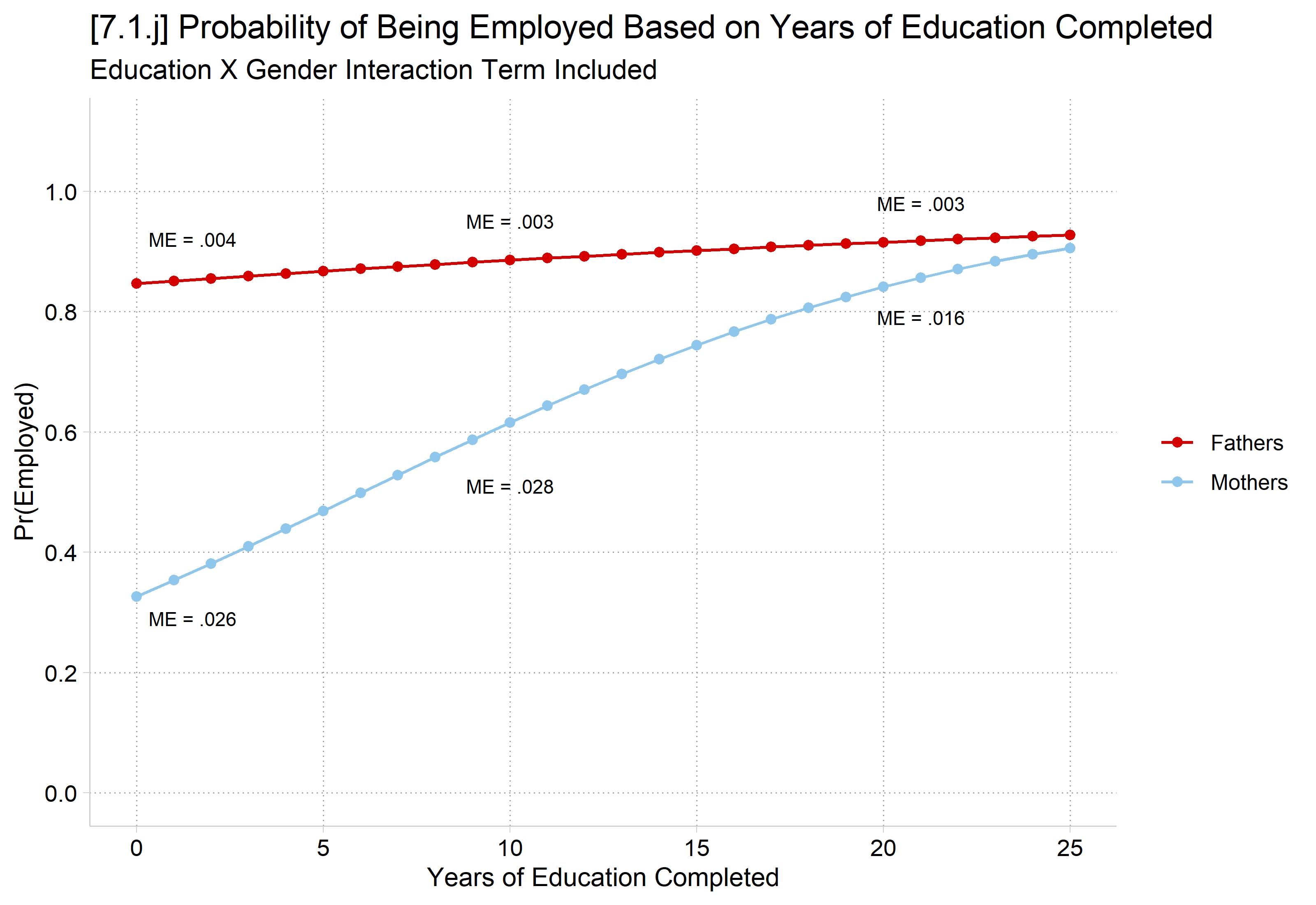
[7.1.j] Predicted probability of being employed by years of education (0 to 25) for fathers and mothers, with an education by gender interaction term. Fathers' probability is nearly flat, from about 0.85 to 0.93 (marginal effects of .004 and .003); mothers' probability rises from about 0.33 to 0.91 (marginal effects of .026 at 0 years, .028 at 10 years, and .016 at 20 years).

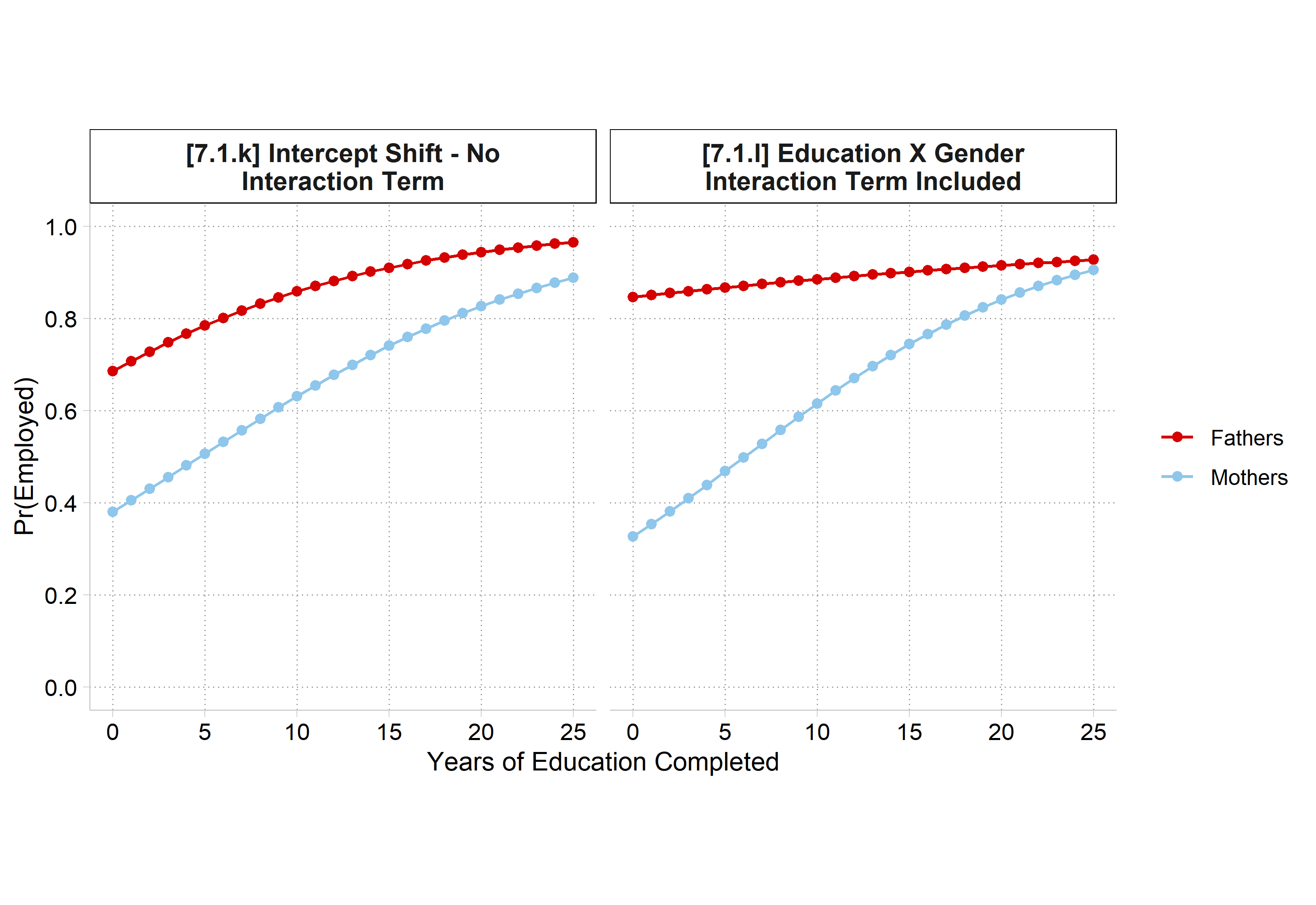
*7.1.k & 7.1.l - Combine plots
est restore intshift
(results intshift are active now)
qui margins, at(edyrs=(0(1)25) woman=(0 1))
marginsplot, noci legend(order(1 "Fathers" 2 "Mothers") position(6)) ///
    ytitle("Pr(Employed)") xtitle("Years of Education Completed") ///
    title("[7.1.k] Intercept Shift - No Interaction Term") aspect(1) ///
    ylabel(0(0.2)1) xlabel(0(5)25) saving(intshift, replace)
Variables that uniquely identify margins: edyrs woman
file intshift.gph saved
est restore interact
(results interact are active now)
qui margins, at(edyrs=(0(1)25) woman=(0 1))
marginsplot, noci legend(order(1 "Fathers" 2 "Mothers") position(6)) ///
    ytitle("Pr(Employed)") xtitle("Years of Education Completed") ///
    title("[7.1.l] Education X Gender Interaction Term Included") aspect(1) //
/
    ylabel(0(0.2)1) xlabel(0(5)25) saving(interact, replace)
Variables that uniquely identify margins: edyrs woman
file interact.gph saved
graph combine intshift.gph interact.gph

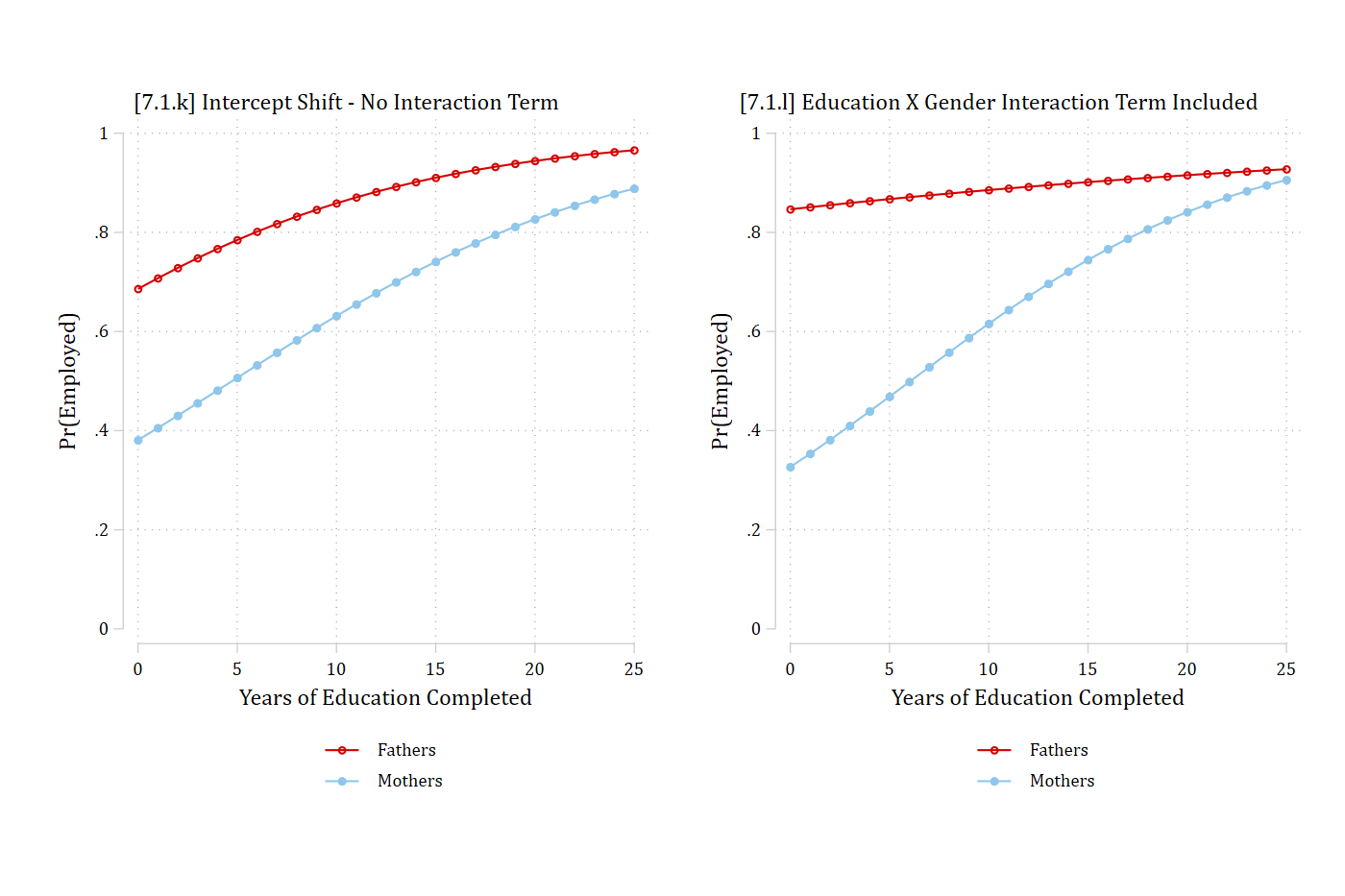
[7.1.k and 7.1.l] Side-by-side predicted probabilities of being employed by years of education (0 to 25) for fathers and mothers. Left, with no interaction term: fathers' curve rises from about 0.69 to 0.96 and mothers' from about 0.38 to 0.89. Right, with the interaction term: fathers' curve is nearly flat near 0.85 to 0.93, and mothers' rises steeply from about 0.33 to 0.91.

# 7.1.k & 7.1.l - Combine plots
pr <- bind_rows(
  "[7.1.k] Intercept Shift - No Interaction Term" = pr_ed(intshift, 0:25),
  "[7.1.l] Education X Gender Interaction Term Included" = pr_ed(interact, 0:25),
  .id = "model")

ggplot(pr, aes(x = edyrs, y = estimate, color = woman)) +
  geom_line() +
  geom_point() +
  facet_wrap(~ model, labeller = label_wrap_gen(35)) +
  scale_x_continuous(breaks = seq(0, 25, 5)) +
  scale_y_continuous(breaks = seq(0, 1, .2), limits = c(0, 1)) +
  labs(x = "Years of Education Completed", y = "Pr(Employed)", color = NULL) +
  theme(aspect.ratio = 1)

[7.1.k and 7.1.l] Side-by-side predicted probabilities of being employed by years of education (0 to 25) for fathers and mothers. Left, with no interaction term: fathers' curve rises from about 0.69 to 0.96 and mothers' from about 0.38 to 0.89. Right, with the interaction term: fathers' curve is nearly flat near 0.85 to 0.93, and mothers' rises steeply from about 0.33 to 0.91.

Is the interaction (product) term necessary?

  • There has been an intense debate in the methodological literature as to whether it is appropriate to discuss interaction effects absent an interaction (product) term in the model
  • The takeaway from this research is: if you want to test for interaction, you should include the product term in the model*
    • Not including the product term can lead to Type I (false positives) or Type II errors (false negatives). See Rainey 2016
  • For more details, see Appendix A7.1 and/or Mize 2019

*If you test for interaction and find none, I see no issue with dropping the product term from subsequent models if you are not testing for interaction in them

Difference in log odds ≠ difference in probs.

  • Remember the coefficients summarize effects in log odds
    • For a binary IV, this is simply the (conditional) difference between the two groups
    • Differences in the probabilities (observed proportions) can be quite different than differences in the log odds
// 7.1.m & 7.1.n - Log odds diff =/= diff in probabilities
clear all
*7.1m: three equal +.10 changes in probability, shown as odds and log-odds
input p0 p1
            p0         p1
  1. .05 .15
  2. .45 .55
  3. .85 .95
  4. end
gen odds0 = p0/(1-p0)
gen odds1 = p1/(1-p1)
gen lo0   = logit(p0)
gen lo1   = logit(p1)
gen oddsratio = odds1/odds0
gen lab_odds  = "+" + string(odds1 - odds0, "%4.2f")
gen lab_lo    = "+" + string(lo1 - lo0, "%4.2f")
twoway (function y = x/(1-x), range(0 .95) pstyle(p1))                     ///
       (pcspike odds0 p0 odds0 p1, pstyle(p2) lpattern(dash))               //
/
       (pcspike odds0 p1 odds1 p1, pstyle(p2) lwidth(thick))                //
/
       (scatter odds0 p0, pstyle(p2))                                       //
/
       (scatter odds1 p1, pstyle(p2) mlabel(lab_odds) mlabposition(11)),    //
/
       title("How odds change for + 0.10 increase in probability") ///
       xtitle("Probability") ytitle("Odds")                   ///
       xlabel(0(.2)1) ylabel(0(5)20) legend(off) name(g_odds, replace)
twoway (function y = logit(x), range(.01 .99) pstyle(p1))                  ///
       (pcspike lo0 p0 lo0 p1, pstyle(p2) lpattern(dash))                   //
/
       (pcspike lo0 p1 lo1 p1, pstyle(p2) lwidth(thick))                    //
/
       (scatter lo0 p0, pstyle(p2))                                         //
/
       (scatter lo1 p1, pstyle(p2) mlabel(lab_lo) mlabposition(11)),        //
/
       title("How log-odds change for a + 0.10 increase in probability") ///
       xtitle("Probability") ytitle("Log-odds")           ///
       xlabel(0(.2)1) ylabel(-4(2)4) legend(off) name(g_lo, replace)
graph combine g_odds g_lo, rows(1) xsize(8) ysize(4)                       ///
    note("Each blue triangle is the same +.10 change in probability.") ///
    title("[7.1.m] Change in log odds / odds does not equal change in probabil
ity")

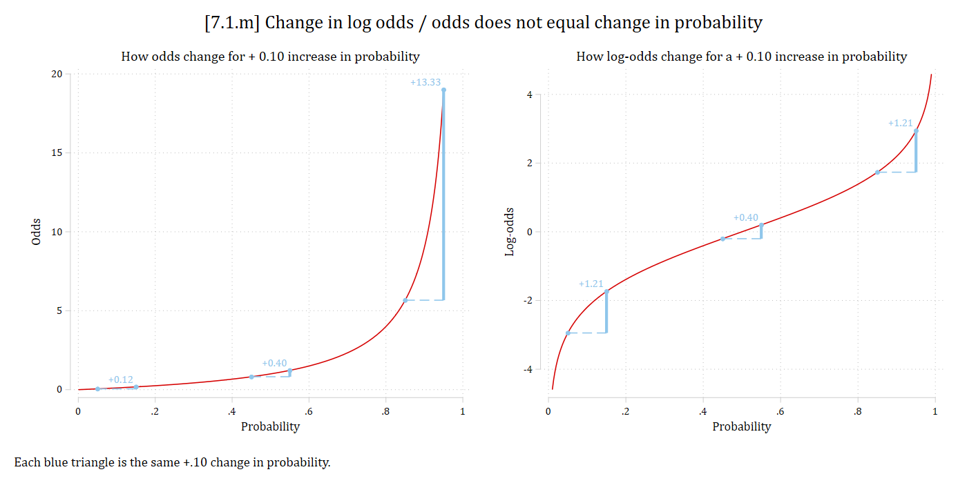
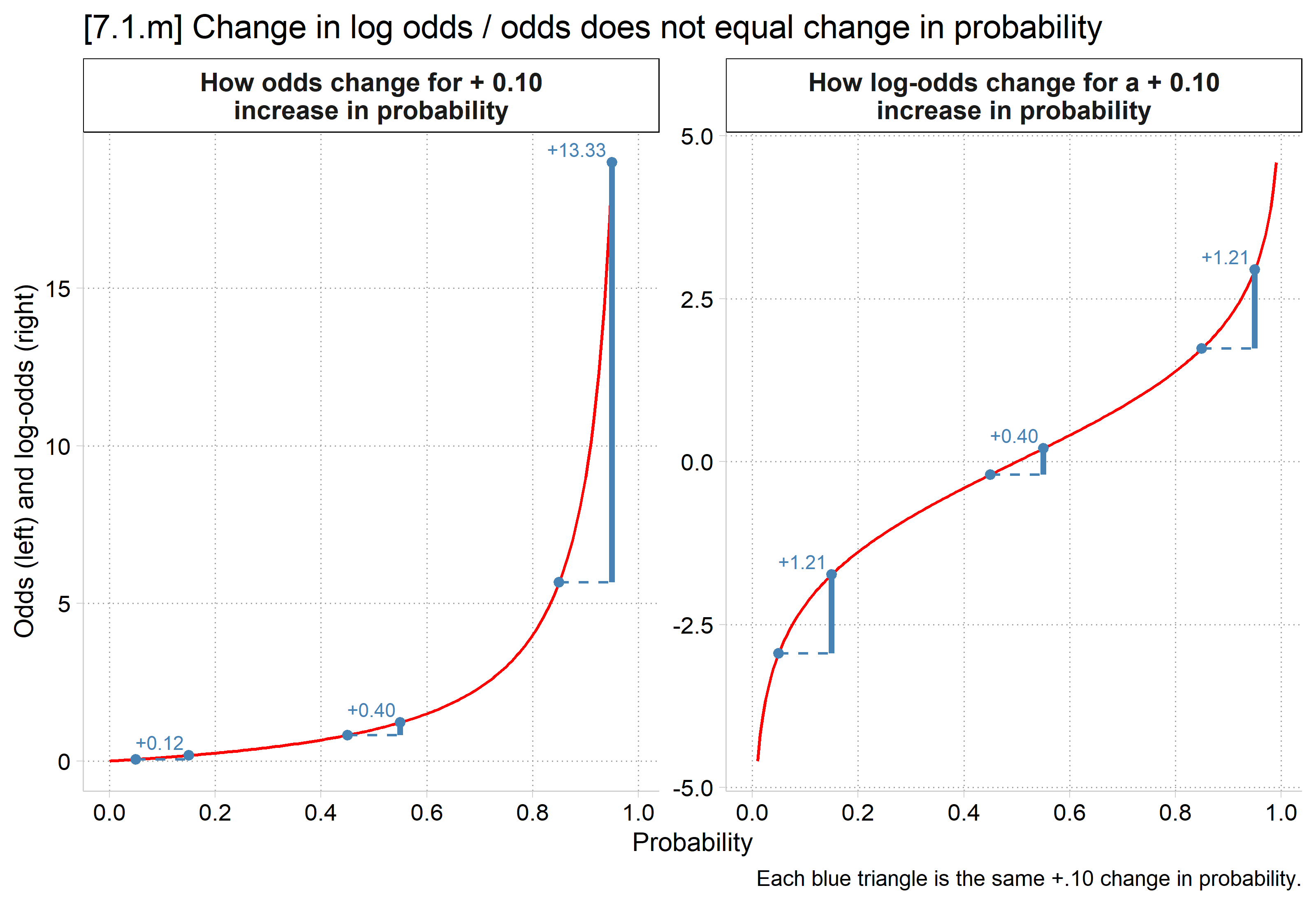
[7.1.m] Two panels showing the same +.10 change in probability at three places (.05 to .15, .45 to .55, and .85 to .95). Left, on the odds curve: the odds change by +0.12, +0.40, and +13.33. Right, on the log-odds curve: the log-odds change by +1.21, +0.40, and +1.21.

# 7.1.m & 7.1.n - Log odds diff =/= diff in probabilities
# 7.1.m: three equal +.10 changes in probability, shown as odds and log-odds
pp <- data.frame(p0 = c(.05, .45, .85), p1 = c(.15, .55, .95))

podds <- "How odds change for + 0.10 increase in probability"
plo <- "How log-odds change for a + 0.10 increase in probability"
curves <- bind_rows(
  data.frame(panel = podds, p = seq(0, .95, .005)) |> mutate(y = p / (1 - p)),
  data.frame(panel = plo, p = seq(.01, .99, .005)) |> mutate(y = qlogis(p)))
steps <- bind_rows(
  pp |> mutate(panel = podds, y0 = p0 / (1 - p0), y1 = p1 / (1 - p1)),
  pp |> mutate(panel = plo, y0 = qlogis(p0), y1 = qlogis(p1))) |>
  mutate(label = sprintf("+%4.2f", y1 - y0))
curves$panel <- factor(curves$panel, levels = c(podds, plo))
steps$panel <- factor(steps$panel, levels = c(podds, plo))

ggplot() +
  geom_line(data = curves, aes(x = p, y = y), color = "red") +
  geom_segment(data = steps, aes(x = p0, xend = p1, y = y0, yend = y0),
    color = "steelblue", linetype = "dashed") +
  geom_segment(data = steps, aes(x = p1, xend = p1, y = y0, yend = y1),
    color = "steelblue", linewidth = 1.2) +
  geom_point(data = steps, aes(x = p0, y = y0), color = "steelblue") +
  geom_point(data = steps, aes(x = p1, y = y1), color = "steelblue") +
  geom_text(data = steps, aes(x = p1, y = y1, label = label), color = "steelblue",
    hjust = 1.1, vjust = -.4, size = 3) +
  facet_wrap(~ panel, scales = "free_y", labeller = label_wrap_gen(35)) +
  scale_x_continuous(breaks = seq(0, 1, .2)) +
  labs(title = "[7.1.m] Change in log odds / odds does not equal change in probability",
    caption = "Each blue triangle is the same +.10 change in probability.",
    x = "Probability", y = "Odds (left) and log-odds (right)")
[7.1.m] Two panels showing the same +.10 change in probability at three places (.05 to .15, .45 to .55, and .85 to .95). Left, on the odds curve: the odds change by +0.12, +0.40, and +13.33. Right, on the log-odds curve: the log-odds change by +1.21, +0.40, and +1.21.

*7.1.n: bar charts for a binary x binary interaction, in log-odds and probabil
ity
* Row 1 = values; row 2 = label positions (12 = above the bar, 6 = below a neg
ative bar)
* Scenario 1: same effect of evidence in log-odds (+2.5) for both groups
matrix s1_lo_A = (-1.5, 1.0 \ 6, 12)
matrix s1_lo_B = ( 0.5, 3.0 \ 12, 12)
matrix s1_p_A  = (invlogit(-1.5), invlogit(1.0))
matrix s1_p_B  = (invlogit( 0.5), invlogit(3.0))
* Scenario 2: same effect of evidence in probability (+.40) for both groups
matrix s2_p_A  = (.20, .60)
matrix s2_p_B  = (.55, .95)
matrix s2_lo_A = (logit(.20), logit(.60) \ 6, 12)
matrix s2_lo_B = (logit(.55), logit(.95) \ 12, 12)
foreach m in s1_lo_A s1_lo_B s1_p_A s1_p_B s2_p_A s2_p_B s2_lo_A s2_lo_B {
    matrix colnames `m' = noev ev
}
local opts vertical recast(bar) barw(0.3) noci mlabel(string(@b, "%3.2f")) ///
    xlab(1 "No evidence" 2 "Evidence") legend(ring(0) position(11) cols(1))
coefplot (matrix(s1_lo_A), aux(2) label("Group A"))                         //
/
         (matrix(s1_lo_B), aux(2) label("Group B")),                        //
/
    `opts' mlabvposition(@aux1) title("No interaction in log-odds")         //
/
    ytitle("Log-odds") ylab(-2(1)4) name(g_s1_lo, replace)
coefplot (matrix(s1_p_A), label("Group A")) (matrix(s1_p_B), label("Group B"))
, ///
    `opts' mlabposition(12) title("...but an interaction in probability")   //
/
    ytitle("Probability") ylab(0(.2)1, format(%2.1f)) yscale(range(0 1.05)) //
/
    name(g_s1_p, replace)
coefplot (matrix(s2_lo_A), aux(2) label("Group A"))                         //
/
         (matrix(s2_lo_B), aux(2) label("Group B")),                        //
/
    `opts' mlabvposition(@aux1) title("An interaction in log-odds")         //
/
    ytitle("Log-odds") ylab(-2(1)4) name(g_s2_lo, replace)
coefplot (matrix(s2_p_A), label("Group A")) (matrix(s2_p_B), label("Group B"))
, ///
    `opts' mlabposition(12) title("...but no interaction in probability")   //
/
    ytitle("Probability") ylab(0(.2)1, format(%2.1f)) yscale(range(0 1.05)) //
/
    name(g_s2_p, replace)
graph combine g_s1_lo g_s1_p g_s2_lo g_s2_p, rows(2) xsize(7) ysize(5) ///
    title("[7.1.n] Interactions can exist in log odds but not probs. (and vice
 versa)")

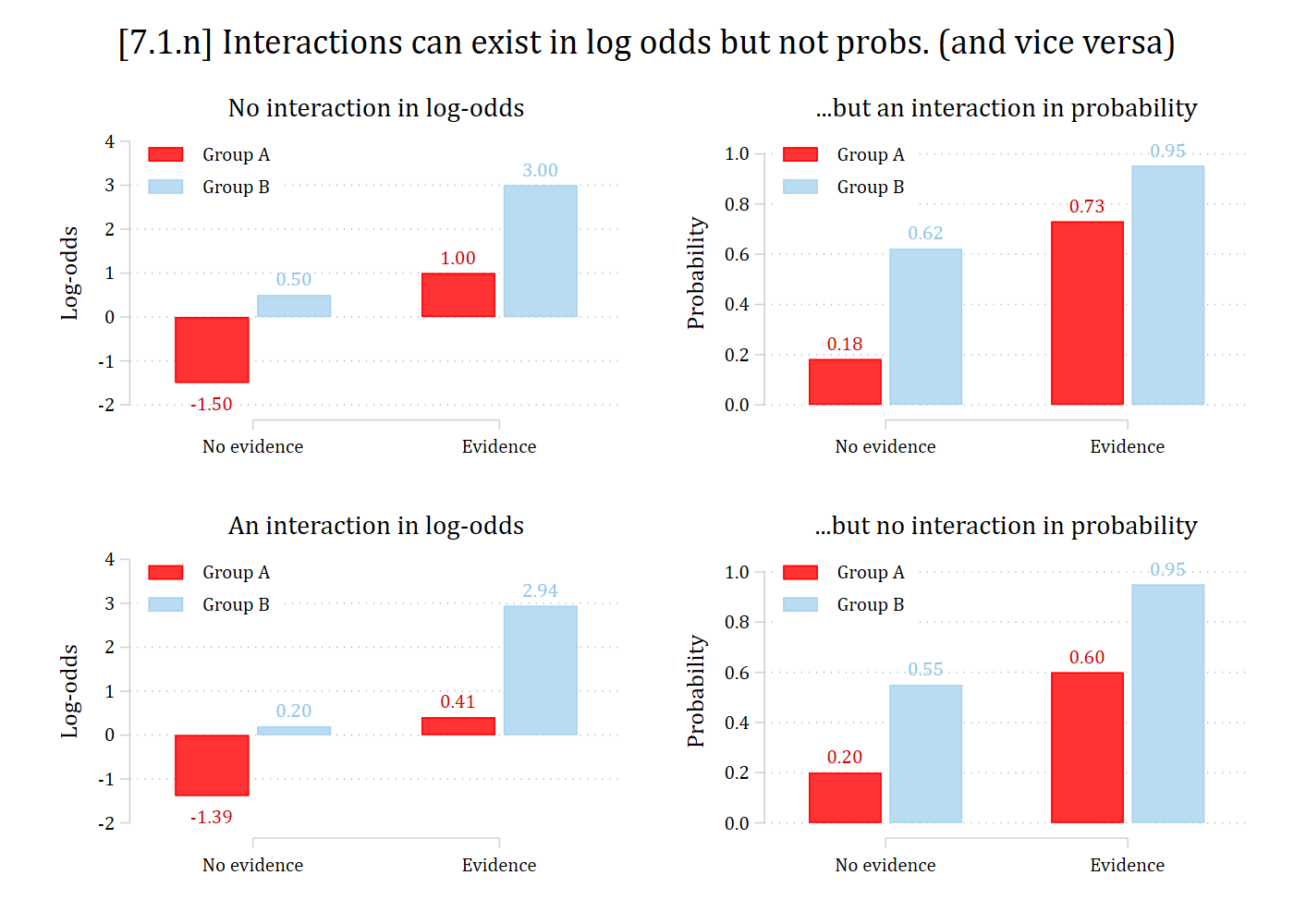
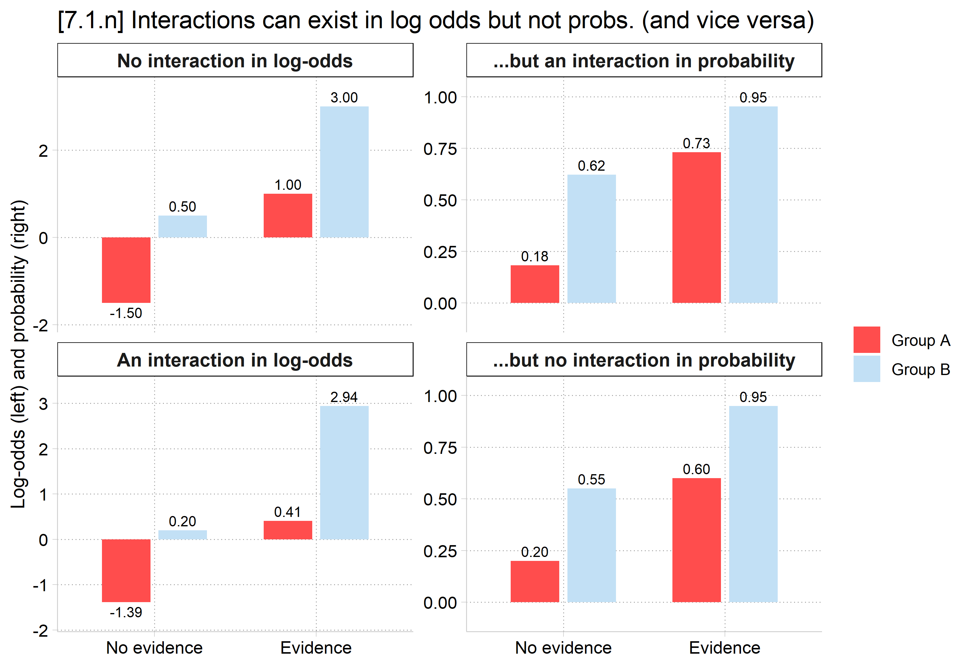
[7.1.n] Four bar charts for groups A and B with and without evidence. Top row: log-odds of -1.50 and 1.00 for group A and 0.50 and 3.00 for group B, the same +2.5 change for both groups (no interaction in log-odds), but the probabilities are 0.18 and 0.73 for A and 0.62 and 0.95 for B, changes of .55 and .33 (an interaction in probability). Bottom row: log-odds of -1.39 and 0.41 for A and 0.20 and 2.94 for B (an interaction in log-odds), but probabilities of 0.20 and 0.60 for A and 0.55 and 0.95 for B, the same +.40 change for both groups (no interaction in probability).

# 7.1.n: bar charts for a binary x binary interaction, in log-odds and probability
# Scenario 1: same effect of evidence in log-odds (+2.5) for both groups
# Scenario 2: same effect of evidence in probability (+.40) for both groups
s1_lo <- c(-1.5, 1.0, 0.5, 3.0)
s2_p <- c(.20, .60, .55, .95)
panels <- c("No interaction in log-odds", "...but an interaction in probability",
  "An interaction in log-odds", "...but no interaction in probability")
bars <- data.frame(
  panel = rep(panels, each = 4),
  group = rep(rep(c("Group A", "Group B"), each = 2), 4),
  evidence = rep(c("No evidence", "Evidence"), 8),
  value = c(s1_lo, plogis(s1_lo), qlogis(s2_p), s2_p)) |>
  mutate(panel = factor(panel, levels = panels),
    evidence = factor(evidence, levels = c("No evidence", "Evidence")))

ggplot(bars, aes(x = evidence, y = value, fill = group)) +
  geom_col(position = position_dodge(.7), width = .6) +
  geom_text(aes(label = sprintf("%3.2f", value), vjust = ifelse(value < 0, 1.4, -.4)),
    position = position_dodge(.7), size = 3) +
  facet_wrap(~ panel, scales = "free_y") +
  scale_y_continuous(expand = expansion(mult = .15)) +
  labs(title = "[7.1.n] Interactions can exist in log odds but not probs. (and vice versa)",
    x = NULL, y = "Log-odds (left) and probability (right)", fill = NULL)

[7.1.n] Four bar charts for groups A and B with and without evidence. Top row: log-odds of -1.50 and 1.00 for group A and 0.50 and 3.00 for group B, the same +2.5 change for both groups (no interaction in log-odds), but the probabilities are 0.18 and 0.73 for A and 0.62 and 0.95 for B, changes of .55 and .33 (an interaction in probability). Bottom row: log-odds of -1.39 and 0.41 for A and 0.20 and 2.94 for B (an interaction in log-odds), but probabilities of 0.20 and 0.60 for A and 0.55 and 0.95 for B, the same +.40 change for both groups (no interaction in probability).

  • Given log odds/odds are in a different metric than the probabilities, which should you trust?
    • You didn’t measure or observe log odds!
    • The natural, observed “natural” metric of the data is proportions, which the probabilities model directly (Mize 2019)
  • Methodological guidance across sociology (Mize 2019), political science (Berry et al. 2010), economics (Ai and Norton 2003), psychology (McCabe et al. 2022), and medicine (Shiroshita et al. 2022) is unanimous in recommending interaction be tested in the predicted probabilities
Back to top