1. Look at your data

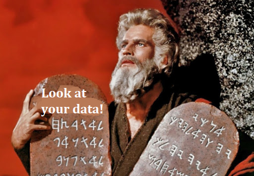
  • The first commandment of data analysis is look at your data
    • Problems and/or quirks with the data are easily ascertained
    • Modeling strategies often become clear only after examining the data

Moses holding a stone tablet that reads: Look at your data!

Histograms

  • Histograms have the advantage of being intuitive and widely used
    • Skew is easy to ascertain via a histogram
  • Histograms “bin” values within a certain range and plot the quantity within that bin as height: higher bars represent ranges that are more frequent in the data

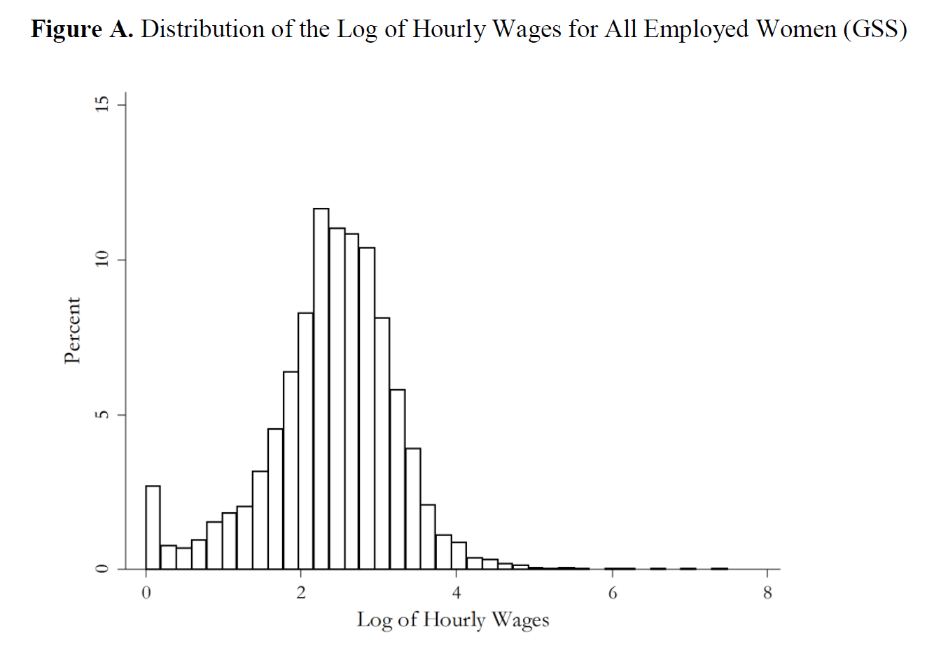
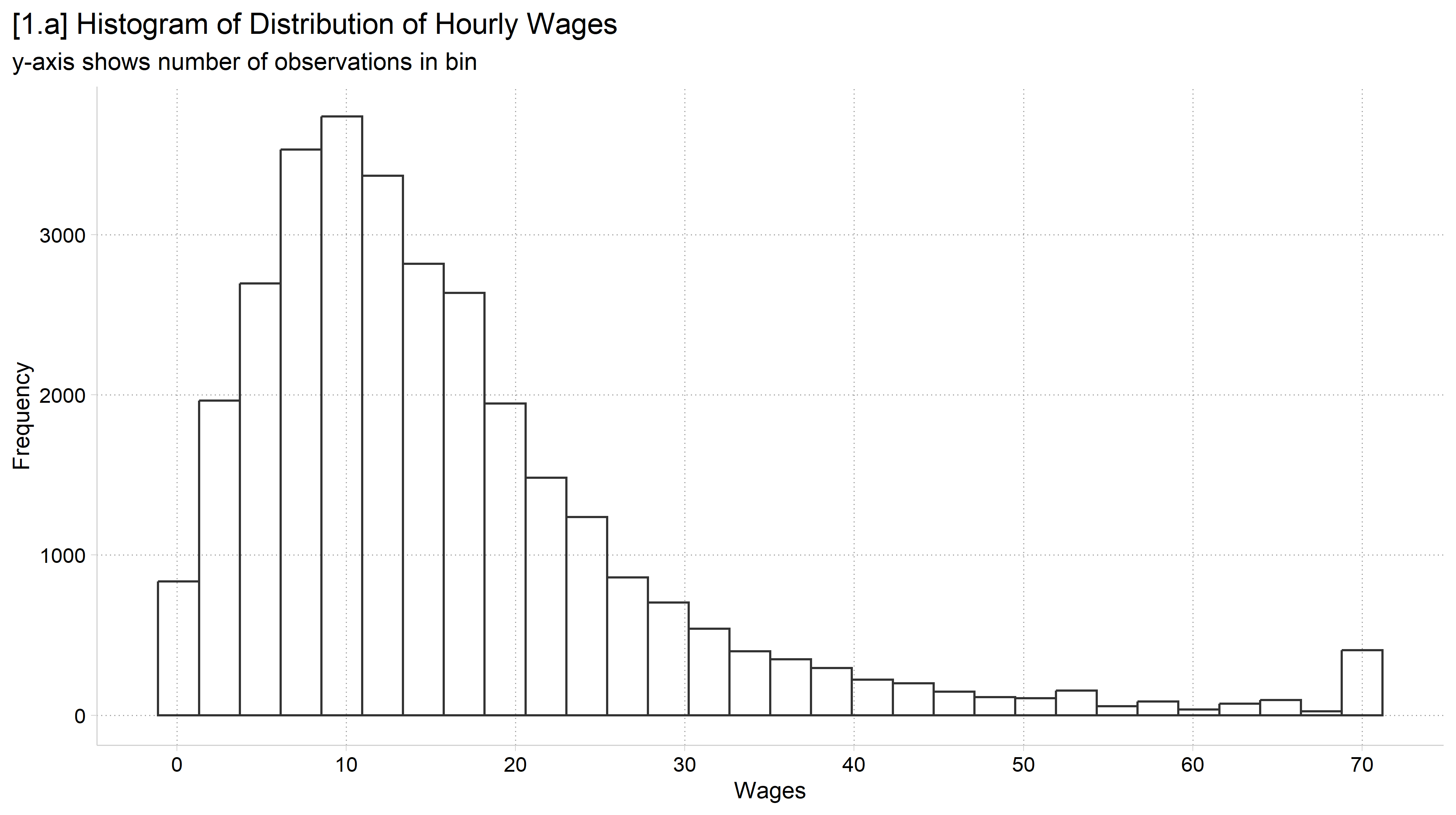
Published histogram: distribution of the log of hourly wages for all employed women in the GSS.

use "https://tdmize.github.io/data/data/gss.dta", clear
(gss.dta | GSS 1972 - 2016 Data | DMV Workshop)
// 1.a - freq option to plot # of obs in each bin
hist wages, freq fcol(none) xlab(0(10)70) ///
    title("[1.a] Histogram of Distribution of Hourly Wages") ///
    subtitle("y-axis shows number of observations in bin")
(bin=44, start=.10516854, width=1.5885189)

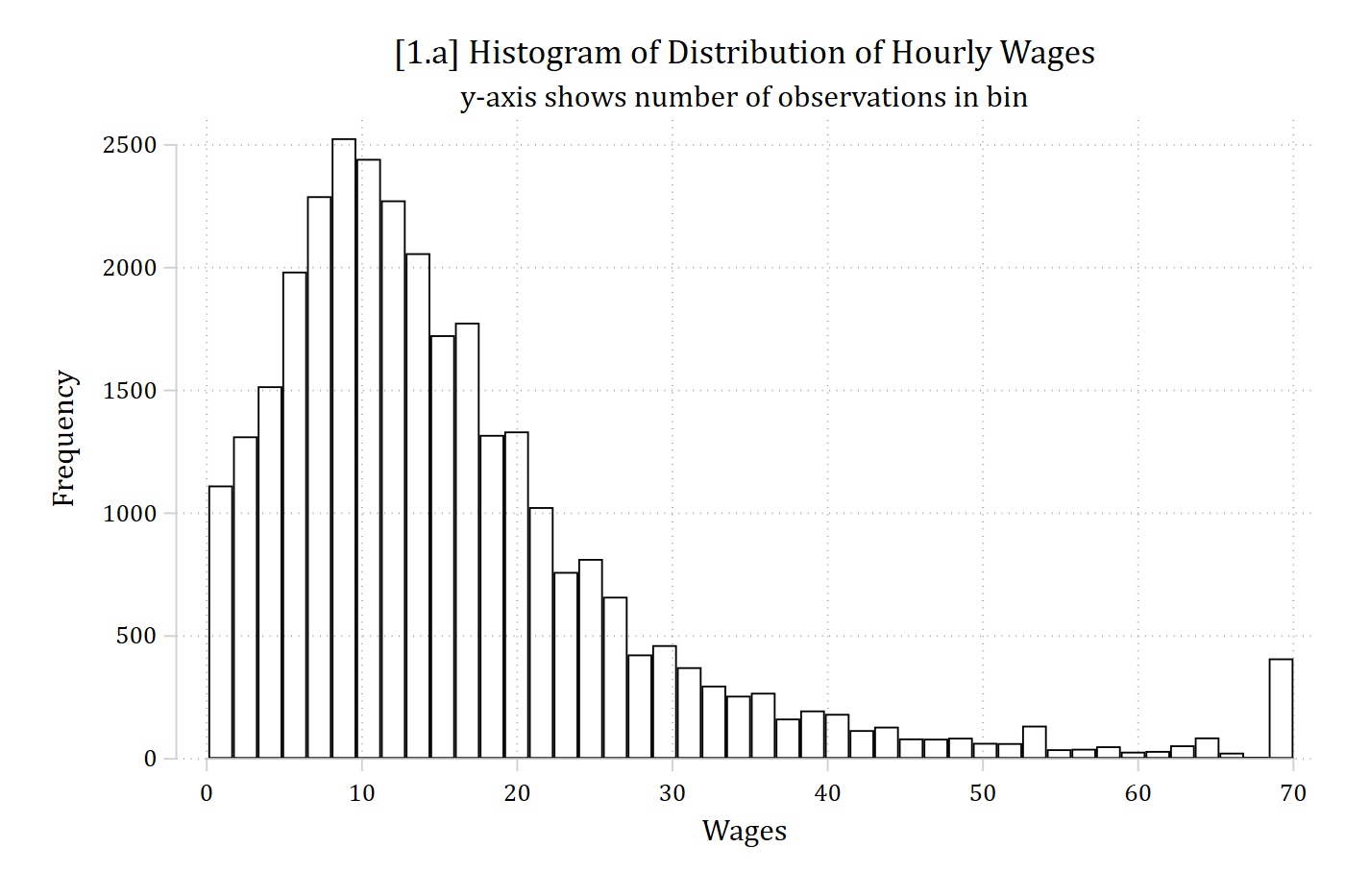
[1.a] Histogram of hourly wages from 0 to 70 with frequency on the y-axis: the distribution is skewed to the right, with most wages between about 5 and 25 and a small spike at the top value of 70.

library(foreign)            # load Stata datasets
library(ggplot2)            # main graphics package
library(dplyr)              # data manipulation tools
library(cleanplots)         # Mize's graphics scheme

## Use cleanplots colors, markers, lines, and theme for all graphs ##
cleanplots_defaults()
theme_update(plot.title.position = "plot")   # titles start at left edge of graph

# General Social Survey Data
gss <- droplevels(read.dta("https://tdmize.github.io/data/data/gss.dta"))

# 1.a - Frequency option to plot # of observations in each bin
ggplot(gss, aes(x = wages)) +
  geom_histogram(fill = NA, color = "gray20") +
  labs(x = "Wages", y = "Frequency",
       title = "[1.a] Histogram of Distribution of Hourly Wages",
       subtitle = "y-axis shows number of observations in bin") +
  scale_x_continuous(breaks = seq(0, 70, 10))
[1.a] Histogram of hourly wages from 0 to 70 with frequency on the y-axis: the distribution is skewed to the right, with most wages between about 5 and 25 and a small spike at the top value of 70.

Kernel density plots

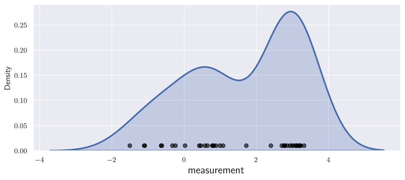
  • Kernel density plots provide smoothed lines showing the distribution of a variable
    • Think of these as a smoothed histogram
    • Rather than the height of individual bins at different values showing frequency/percent, the height of the smooth line illustrates density of the data at that value
      • NOTE: density ≈ proportion of observations near that value

A kernel density curve drawn over a row of individual data points: the curve is highest where the points are most concentrated.

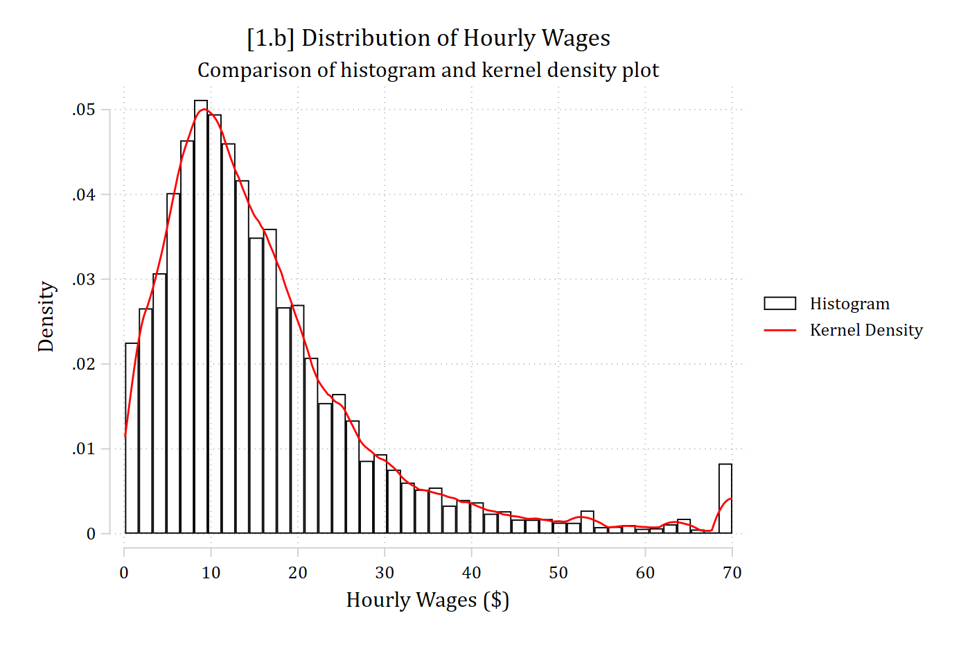
// 1.b - Overlay a kernel density plot on a histogram to illustrate what it do
es
*NOTE: Just pedagogical, not a graph you would usually make
twoway ///
    hist     wages, fcol(none) || ///
    kdensity wages, col(red)   || ///
    , xlab(0(10)70) legend(order(1 "Histogram" 2 "Kernel Density")) ///
    ytitle("Density") xtitle("Hourly Wages ($)") ///
    title("[1.b] Distribution of Hourly Wages") ///
    subtitle("Comparison of histogram and kernel density plot")

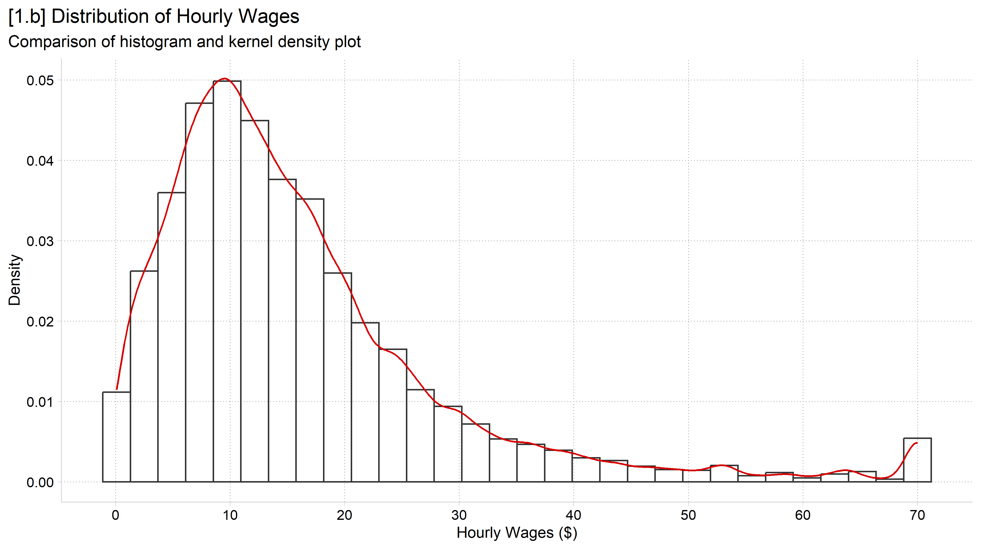
[1.b] Histogram of hourly wages on the density scale with a red kernel density line overlaid: the smooth line follows the tops of the bars, peaking near 10 dollars and trailing off to the right.

# 1.b - Overlay a kernel density plot on a histogram to illustrate what it does
# NOTE: Just pedagogical, not a graph you would usually make
ggplot(gss, aes(x = wages)) +
  geom_histogram(aes(y = after_stat(density)), fill = NA, color = "gray20") +
  geom_density(color = cleanplots_colors("red")) +
  labs(x = "Hourly Wages ($)", y = "Density",
       title = "[1.b] Distribution of Hourly Wages",
       subtitle = "Comparison of histogram and kernel density plot") +
  scale_x_continuous(breaks = seq(0, 70, 10))
[1.b] Histogram of hourly wages on the density scale with a red kernel density line overlaid: the smooth line follows the tops of the bars, peaking near 10 dollars and trailing off to the right.

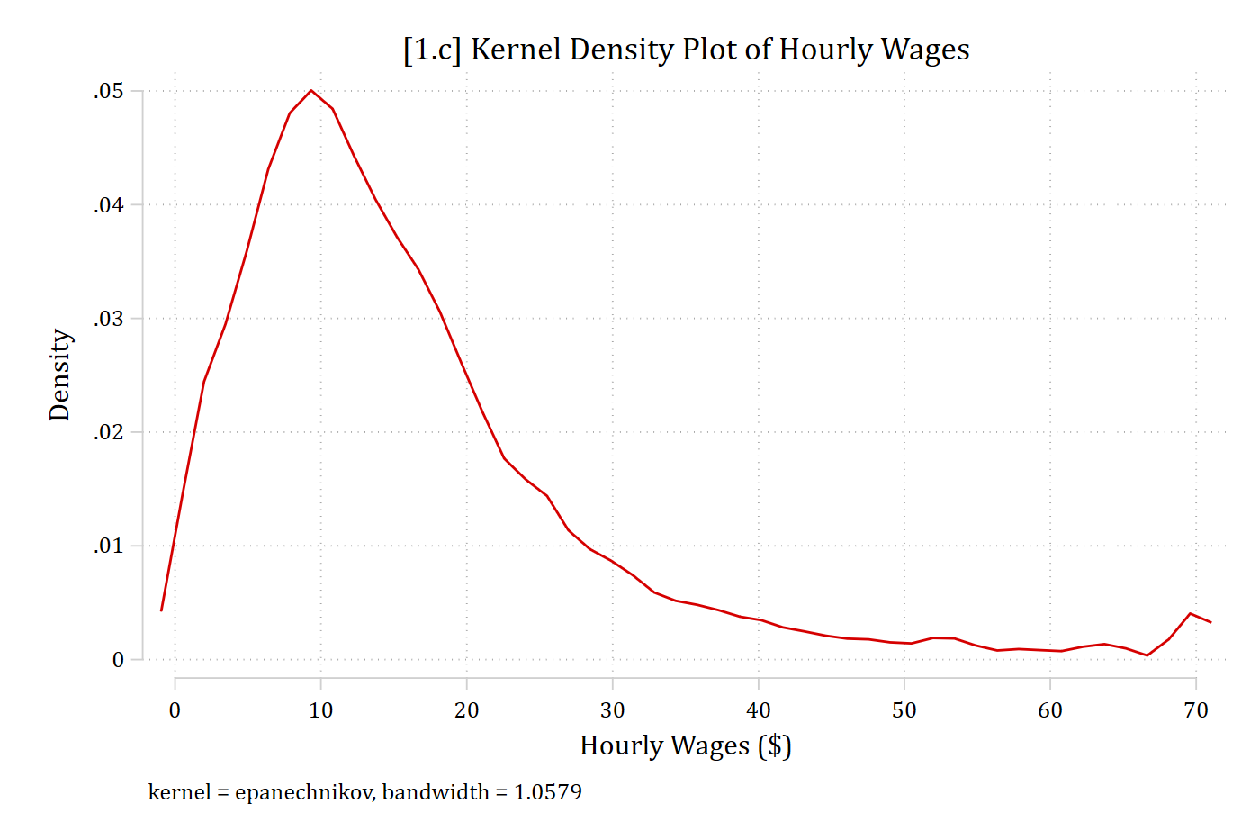
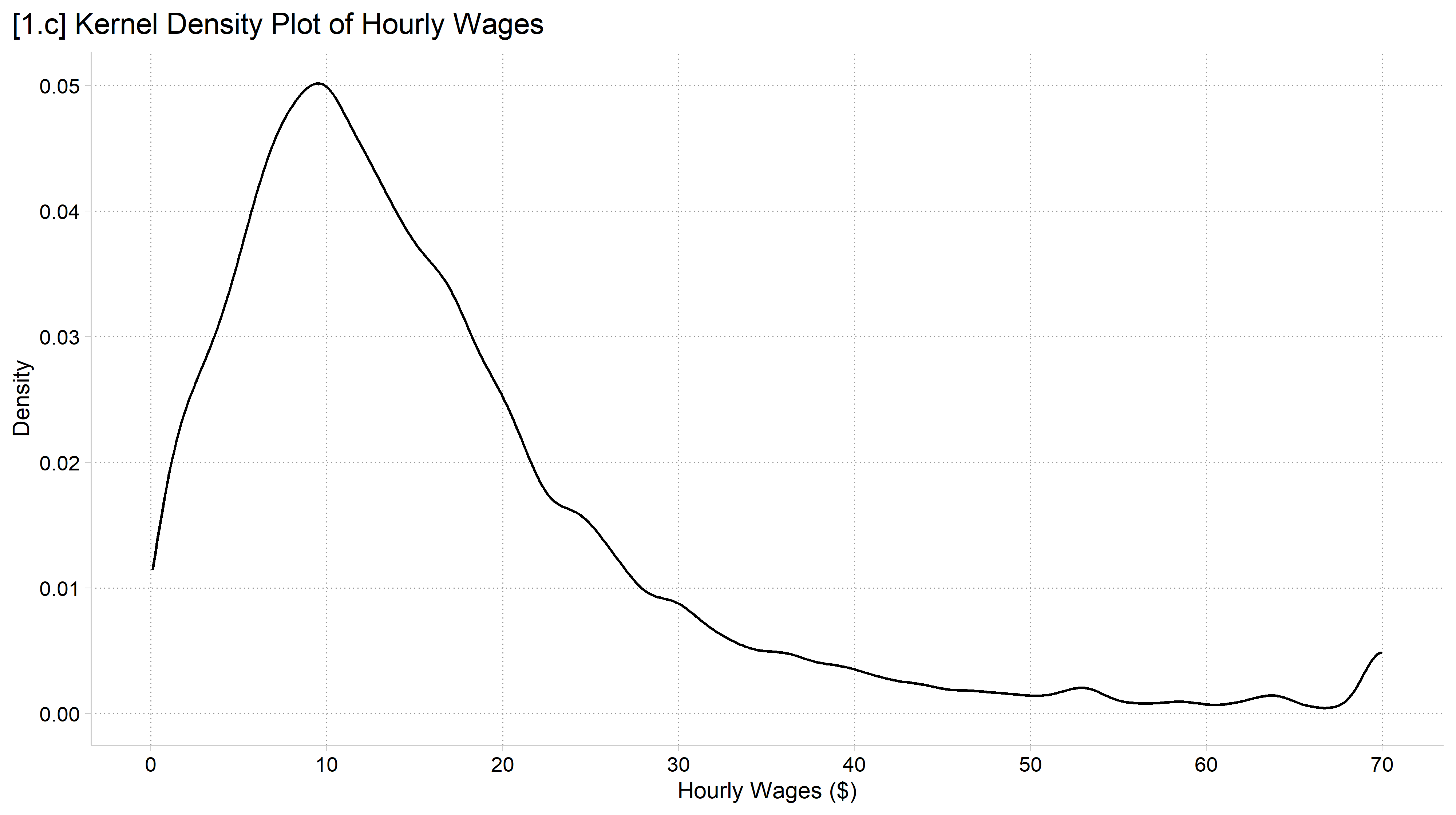
// 1.c - Usually, just want the density and not the histogram too
kdensity wages, xlab(0(10)70) ///
    ytitle("Density") xtitle("Hourly Wages ($)") ///
    title("[1.c] Kernel Density Plot of Hourly Wages")

[1.c] Kernel density plot of hourly wages: the line rises steeply to a peak near 10 dollars and then declines slowly toward 70.

# 1.c - Usually, just want the density and not the histogram too
ggplot(gss, aes(x = wages)) +
  geom_density() +
  labs(x = "Hourly Wages ($)", y = "Density",
       title = "[1.c] Kernel Density Plot of Hourly Wages") +
  scale_x_continuous(breaks = seq(0, 70, 10))
[1.c] Kernel density plot of hourly wages: the line rises steeply to a peak near 10 dollars and then declines slowly toward 70.

Published example

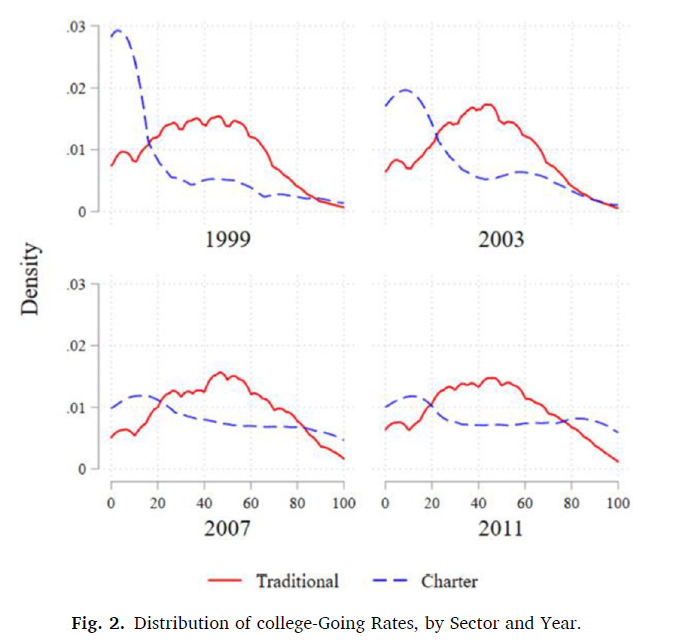
Published figure with four panels (1999, 2003, 2007, 2011), each showing kernel densities of college-going rates for traditional and charter schools.

From Renzulli, Boylan, and Paino 2023

Note, to make multi-panel graphs like this use graph combine in Stata and ggplot2’s faceting features in R

The Methodology Center illustration: small line drawings of graphs around a central MCAP circle.

A person pointing at kernel density curves on a board in front of an audience: the drawing in the Methodology Center illustration.

*Read about The Methodology Center’s graphic

Box (and whisker) plots

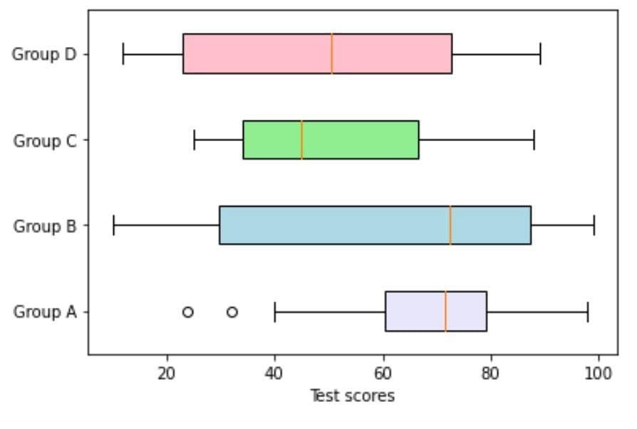
  • Box plots are useful for comparing distributions across variables or across waves (or groups)
    • Standardized rules make comparing distributions easy

Example box plots of test scores for four groups, A through D.

Box and whisker plot rules

  • Rules:
    • Line break in middle of box = median
    • Box boundaries = interquartile range (IQR)
      • IQR: 75th percentile – 25th percentile
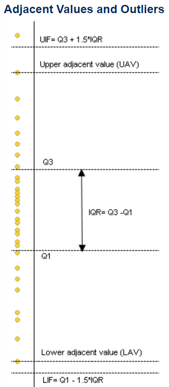
    • Whiskers = range of data without outliers*
      • I.e., Where the vast majority of the data falls
    • Dots = outliers
      • NOTE: Following Tukey (1977), the length of the whiskers (and thus, the cutoff for outliers) is:
        1. Upper cutoff: 75th percentile + 1.5 * IQR
        2. Lower cutoff: 25th percentile - 1.5 * IQR

Diagram of adjacent values and outliers: the quartiles Q1 and Q3, the IQR between them, the upper and lower adjacent values, and the cutoffs Q3 + 1.5 IQR and Q1 - 1.5 IQR.

use "https://tdmize.github.io/data/data/ah_si.dta", clear
(ah-si.dta | Add Health Waves 1-6: Cleaned for MCAP SI)
* Top code drinks in the past year at 1,000
gen numdrinksyrT = numdrinksyr
(432 missing values generated)
recode numdrinksyrT 1000 / 9125 = 1000
(1,649 changes made to numdrinksyrT)
lab var numdrinksyrT "# of drinks last year (top coded at 1,000)"
// 1.d - Drinks in the past year, with separate boxes by wave
graph box numdrinksyrT, over(wave) ///
    ytitle("# of drinks in the past year") ///
    title("[1.d] Box plot of drinks in the past year by wave of Add Health") /
//
    subtitle("Top coded at 1,000 drinks")

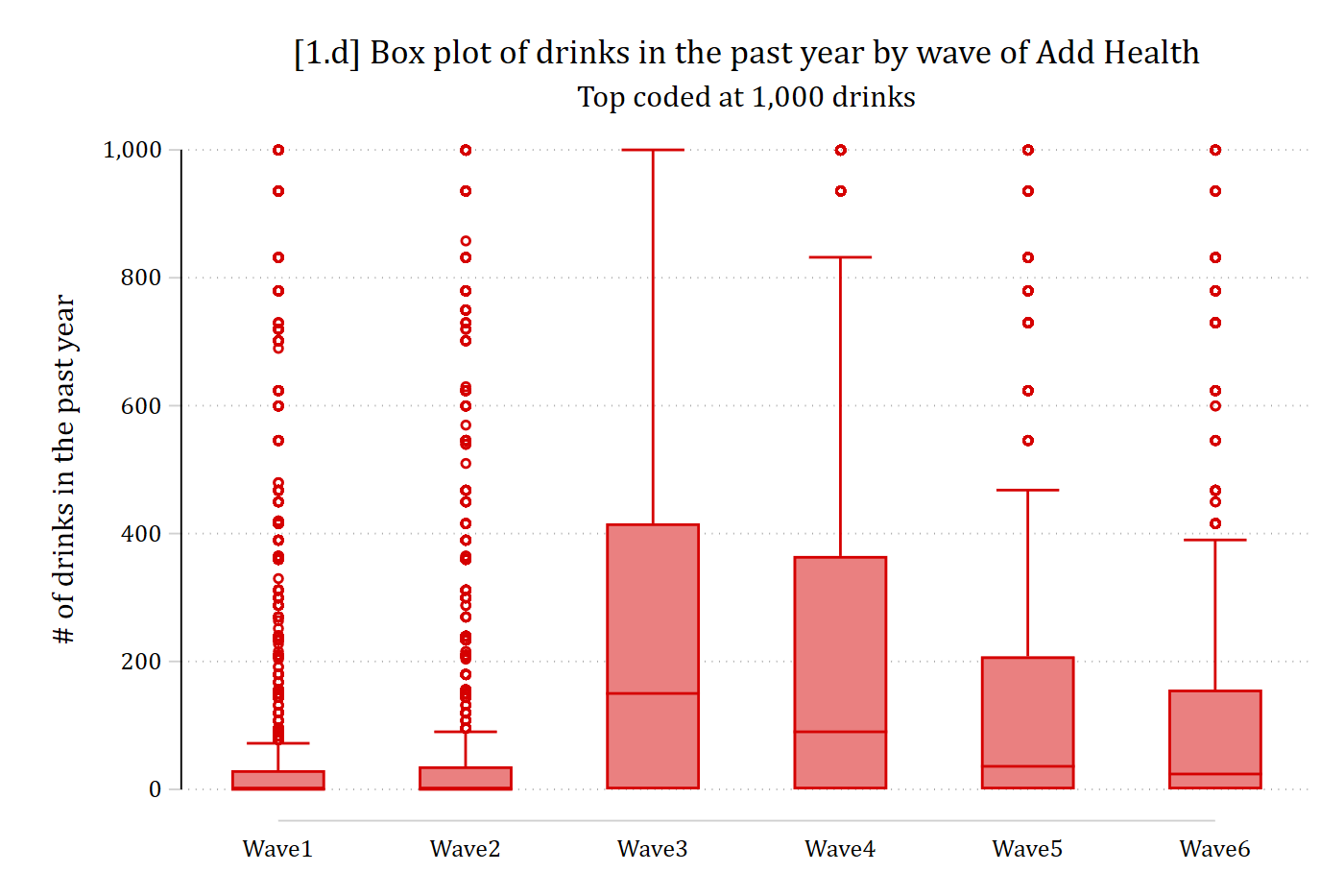
[1.d] Box plots of the number of drinks in the past year for Add Health waves 1 to 6: waves 1 and 2 have very small boxes near zero, waves 3 and 4 have the widest boxes, and every wave has many outliers up to the top code of 1,000.

# Add Health Data
ah <- read.dta("https://tdmize.github.io/data/data/ah_si.dta")

# Top code drinks in the past year at 1,000
ah$numdrinksyrT <- pmin(ah$numdrinksyr, 1000)

# 1.d - Drinks in the past year, with separate boxes by wave
ggplot(ah, aes(x = wave, y = numdrinksyrT)) +
  geom_boxplot() +
  labs(x = "",
       y = "# of drinks in the past year",
       title = "[1.d] Box plot of drinks in the past year by wave of Add Health",
       subtitle = "Top coded at 1,000 drinks")

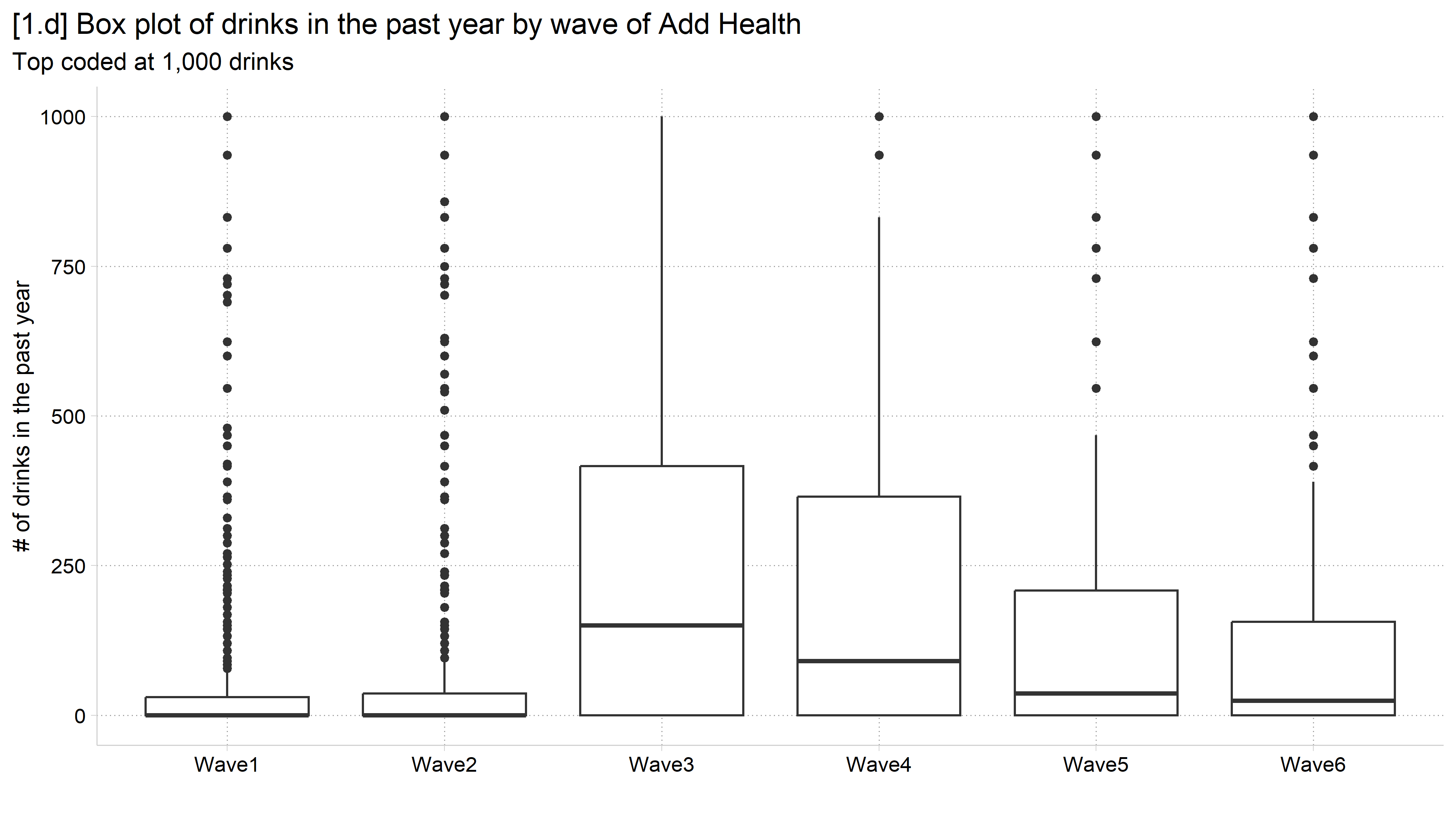
[1.d] Box plots of the number of drinks in the past year for Add Health waves 1 to 6: waves 1 and 2 have very small boxes near zero, waves 3 and 4 have the widest boxes, and every wave has many outliers up to the top code of 1,000.

// 1.e - Add a second grouping variable
graph box numdrinksyrT, ///
    over(male) over(wave) asyvars horizontal ///
    ytitle("# of drinks in the past year") ///
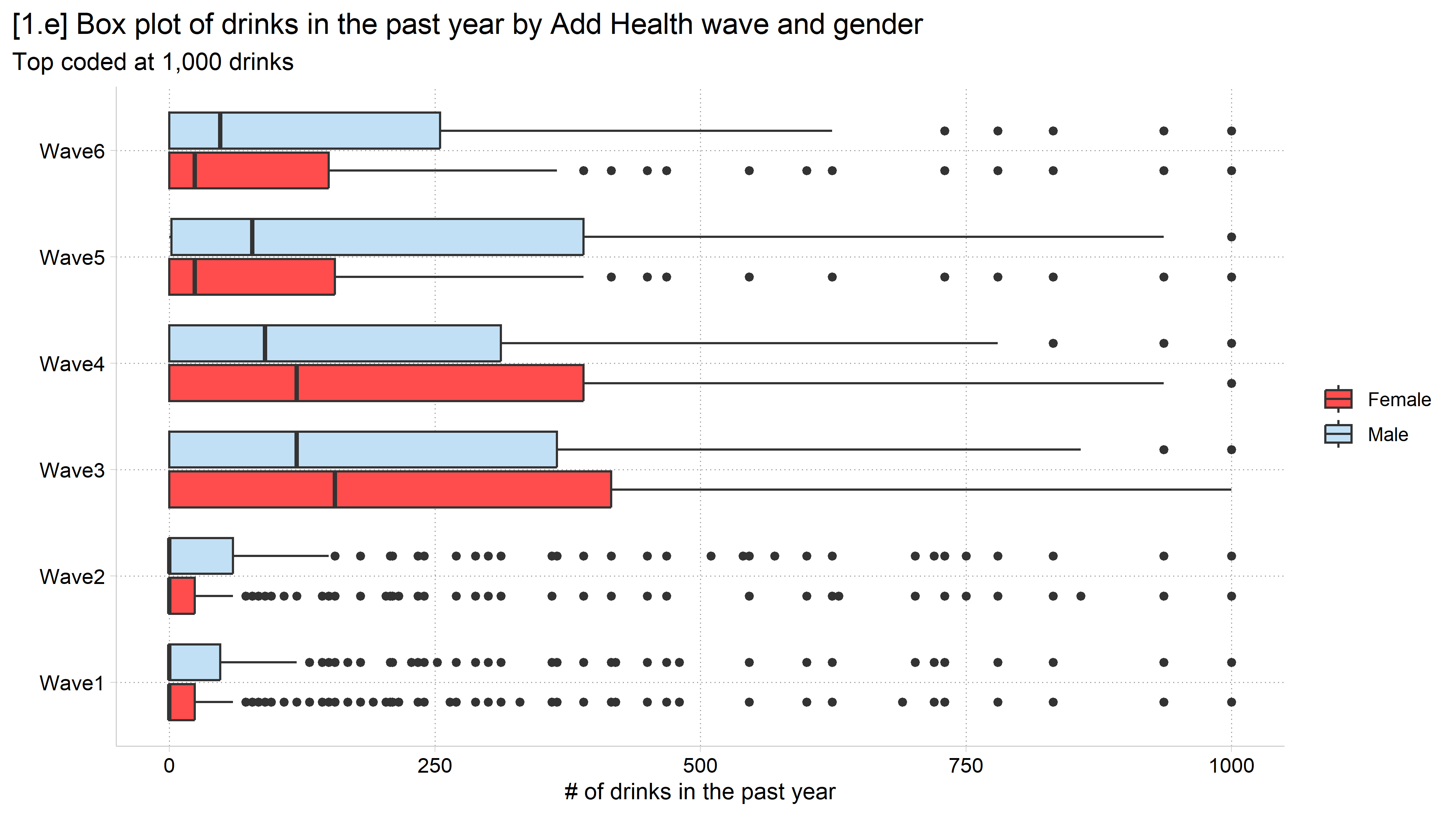
    title("[1.e] Box plot of drinks in the past year by Add Health wave and ge
nder") ///
    subtitle("Top coded at 1,000 drinks")

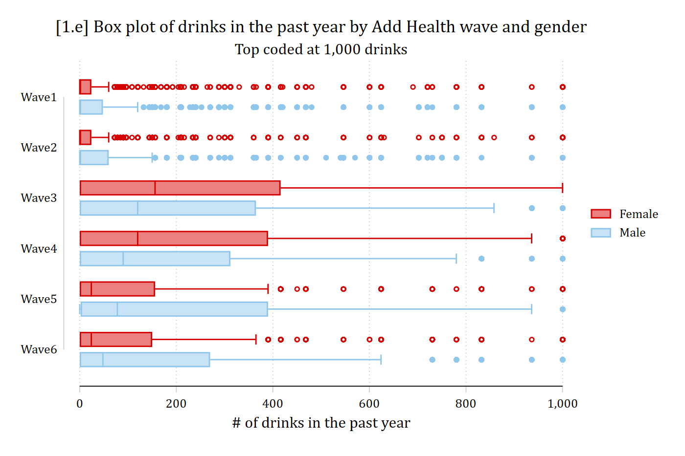
[1.e] Horizontal box plots of drinks in the past year by Add Health wave, with separate red boxes for females and light blue boxes for males: the female boxes are wider in waves 3 and 4 and the male boxes are wider in waves 5 and 6.

# 1.e - Add a second grouping variable
ggplot(filter(ah, !is.na(male)), aes(x = wave, y = numdrinksyrT, fill = male)) +
  geom_boxplot() +
  coord_flip() +
  labs(x = "",
       y = "# of drinks in the past year", fill = "",
       title = "[1.e] Box plot of drinks in the past year by Add Health wave and gender",
       subtitle = "Top coded at 1,000 drinks")

[1.e] Horizontal box plots of drinks in the past year by Add Health wave, with separate red boxes for females and light blue boxes for males: the female boxes are wider in waves 3 and 4 and the male boxes are wider in waves 5 and 6.

Back to top