2.1 Interpretation with Marginal Effects
- A marginal effect is your model’s answer to a counterfactual question:
- If the value of this independent variable were different, how would the predicted outcome change?
- Every marginal effect is an answer to some “what if” question you pose to your fitted model
- If the value of this independent variable were different, how would the predicted outcome change?
- A marginal effect is defined as:
- The predicted change in the outcome for a change in \(x_{k}\) of δ, holding other predictors constant
- And is calculated as the difference between two model predictions (\(\eta\))
- The predicted change in the outcome for a change in \(x_{k}\) of δ, holding other predictors constant
- With nonlinearities, it is often the best choice to provide a summary of the effect of a variable
Marginal effects with linear additive effects
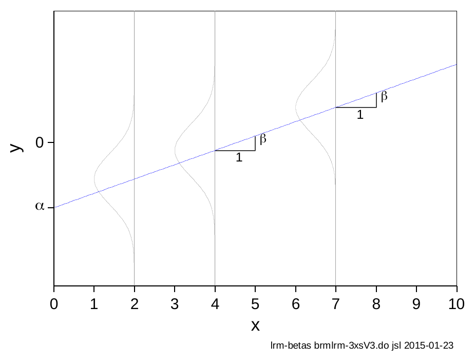
- In the special case of a linear regression model with linear, non-interactive (i.e., additive) effects: \({ME}_{x_{k} + 1} = \beta_{x_{k}}\)
- This is only true in this incredibly limited situation
Marginal effects with nonlinear and/or interactive effects
- Marginal effects are most useful for nonlinear and/or interactive effects
- In these cases, the marginal effects are summarizing different information than the coefficients
Marginal effects defined
- Denote our focal IV as \(x_{k}\)
- Denote the control variables as \(\mathbf{x}_{- k}\) (all other IVs in the model excluding \(x_{k}\))
- A marginal effect, at its simplest, is the difference between two predictions (denoted as \(\eta\) “eta”): one at a starting value of substantive interest; one at an ending value of substantive interest
- Formally:
\[ME = \eta\left( x_{k} = end,\ \mathbf{x}_{- k} = \mathbf{x}^{\mathbf{*}} \right) - \eta\left( x_{k} = start,\ \mathbf{x}_{- k} = \mathbf{x}^{\mathbf{*}} \right)\]
- Starting and ending values of the focal IV \(x_{k}\) can be any values of substantive interest. For binary IVs, there are only two logical choices: 0 and 1
\[{ME}_{binary} = \eta\left( x_{k} = 1,\ \mathbf{x}_{- k} = \mathbf{x}^{\mathbf{*}} \right) - \eta\left( x_{k} = 0,\ \mathbf{x}_{- k} = \mathbf{x}^{\mathbf{*}} \right)\]
- For example, can compare a prediction for no degree (=0) to college (=1)
Marginal effects for continuous IVs
- For continuous IVs, there are many more choices for starting and ending values. Common choices:
- start = mean of \(x_{k}\)
- end = mean + 1
- end = mean + SD is also common*; sometimes more informative
- Any other values of substantive interest can be used for start and end (e.g., age 30 and age 55)
- This flexibility is one of the benefits of using marginal effects for interpretation
Amount of change (\(\delta\))
- There are two types of marginal effects for continuous IVs, differing in the amount of change \(\delta\) (Mize and Han 2026)
- Discrete change in \(\widehat{y}\) as an IV changes by a fixed amount
- E.g., A one unit increase; a standard deviation increase
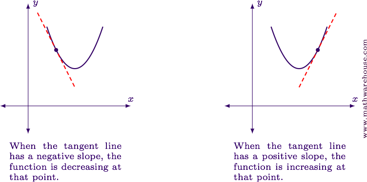
- Instantaneous rate of change in \(\widehat{y}\) (first derivative; AKA slopes)
- Rates of changes are less intuitive to interpret and thus less popular in most social science applications
- Discrete change in \(\widehat{y}\) as an IV changes by a fixed amount
*In most applications, especially for large changes, I recommend centering the change on start value
Terminology is confusing
“Mathematics is the art of giving the same name to different things.” – Henri Poincaré
- I use marginal effects as an umbrella term for all of these effects (i.e., both discrete and rates of changes), regardless of the specific amount of change
- “Marginal” comes from the idea of evaluating a change at the margin—that is, asking what happens to an outcome when a predictor changes slightly, holding other things constant
- Instantaneous rates of changes (AKA slopes) are sometimes called partial effects or (even more confusing) marginal changes
Example: Occupational Prestige
Data is from pooled General Social Survey (GSS) data from 1972 – 2016
use "https://tdmize.github.io/data/data/cda_gss", clear(cda_gss.dta | GSS 1972-2021 CDA - Categorical Data Analysis | date created 202
> 3)hist occprest, percent fcol(none) ylab(0(2)10)(bin=47, start=12, width=1.5744681)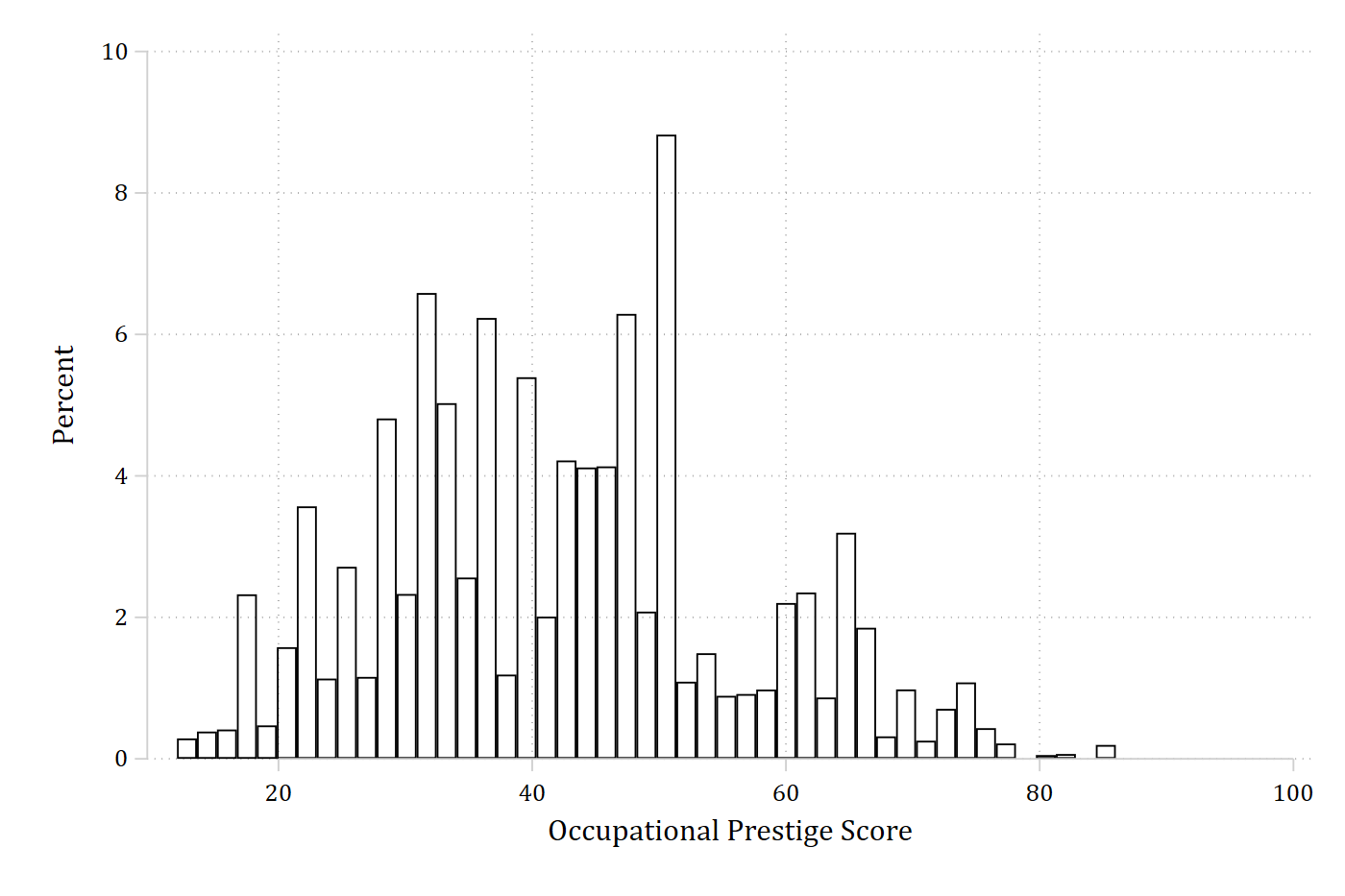
Example occupational prestige scores
- A 2018 ASR article examining occupational prestige scores
- The list of scores for various occupations can be found here. Some examples:
| Occupation | Prestige score |
|---|---|
| Elementary school teachers | 64.08 |
| Sociologists | 60.75 |
| “Sociology teachers” | 73.51 |
| Statisticians | 55.57 |
| Architects | 73.15 |
| Physicians | 86.05 |
| Registered nurses | 66.48 |
| Sales workers, shoes | 27.67 |
| Bartenders | 24.53 |
| Barbers | 35.71 |
| Parking lot attendants | 21.22 |
Regression results for occupational prestige (DV)
regress occprest c.age i.woman i.college Source | SS df MS Number of obs = 58,304
-------------+---------------------------------- F(3, 58300) = 6232.46
Model | 2765051.56 3 921683.852 Prob > F = 0.0000
Residual | 8621657.35 58,300 147.884346 R-squared = 0.2428
-------------+---------------------------------- Adj R-squared = 0.2428
Total | 11386708.9 58,303 195.302281 Root MSE = 12.161
-------------------------------------------------------------------------------
occprest | Coefficient Std. err. t P>|t| [95% conf. interval]
--------------+----------------------------------------------------------------
age | 0.041 0.003 14.027 0.000 0.035 0.047
|
woman |
Women | -0.178 0.101 -1.756 0.079 -0.376 0.021
|
college |
College De.. | 16.422 0.121 136.142 0.000 16.185 16.658
_cons | 36.621 0.157 233.710 0.000 36.314 36.928
-------------------------------------------------------------------------------esttab, b(2) se(2) nobase label ///
title("[2.1.b] Occupational Prestige Based on Age, Gender, and Education")[2.1.b] Occupational Prestige Based on Age, Gender, and Education
------------------------------------
(1)
Occupation~e
------------------------------------
age of respondent 0.04***
(0.00)
Women -0.18
(0.10)
College Degree 16.42***
(0.12)
Constant 36.62***
(0.16)
------------------------------------
Observations 58304
------------------------------------
Standard errors in parentheses
* p<0.05, ** p<0.01, *** p<0.001qui margins woman, at(age=(20(5)80))
marginsplot, ///
recastci(rline) ciopts(lpat(dash) col(gs12)) ylab(38(2)46) ///
title("[2.1.c] Predicted Occupational Prestige Based on Person's Age", siz
e(medium)) ///
ytitle("Occupational Prestige")Variables that uniquely identify margins: age woman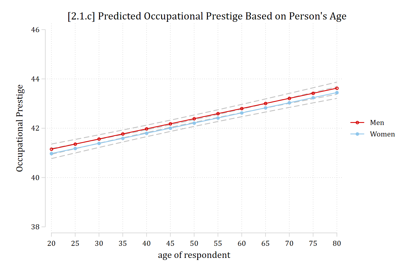
Calculating marginal effects
\[\widehat{occprest} = 36.63 + 0.04*{age}_{i} - 0.183*{woman}_{i} + 16.43*{college}_{i}\]
To calculate the marginal effect of age, where should we hold the other variables constant?
Calculate the effect of aging from 40 to 50 for women without college degrees:
\(\widehat{occprest} = 36.63 + 0.04*40 - 0.183*1 + 16.43*0\) = 38.047
\(\widehat{occprest} = 36.63 + 0.04*50 - 0.183*1 + 16.43*0\) = 38.447
38.447 – 38.047 = 0.400
Calculate the effect of aging from 40 to 50 for women with college degrees:
\(\widehat{occprest} = 36.63 + 0.04*40 - 0.183*1 + 16.43*1\) = 54.477
\(\widehat{occprest} = 36.63 + 0.04*50 - 0.183*1 + 16.43*1\) = 54.877
54.877 – 54.477 = 0.400
di 36.63 + 0.04*40 - 0.183*1 + 16.43*038.047di 36.63 + 0.04*50 - 0.183*1 + 16.43*038.447di 38.447 - 38.047.4di 36.63 + 0.04*40 - 0.183*1 + 16.43*154.477di 36.63 + 0.04*50 - 0.183*1 + 16.43*154.877di 54.877 - 54.477.4Simple interpretation due to linearity
Continuous variables
- Interpretation: for a unit increase in xk the expected change in y is ME, holding other variables constant
- Remember, in the case of linear additive effects in linear regression: \({ME}_{x_{k} + 1} = \beta_{x_{k}}\)
For each additional year a person ages, their job prestige is expected to be 0.04 points higher, holding other variables constant
For ten additional years of age, a person’s job prestige is expected to increase by 0.4 points, holding other variables constant
Note: 0.04 * 10 = 0.40
Plot the effects for women, separately for those who went to college or not:
qui margins, at(age=(20(5)90) woman=(1) college=(0 1))
marginsplot, ///
    recastci(rline) ciopts(lpat(dash) col(gs12)) ylab(35(5)60) ///
    title("[2.1.d] Predicted Occupational Prestige Based on Person's Age", siz
e(medium)) ///
    subtitle("Women Respondents Only", size(medium)) ///
    ytitle("Occupational Prestige")
Variables that uniquely identify margins: age college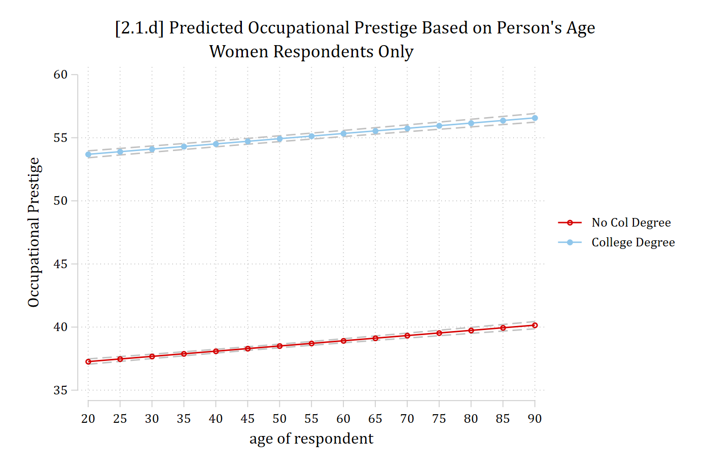
Calculating marginal effects for a binary variable
\[\widehat{occprest} = 36.63 + 0.04*{age}_{i} - 0.183*{woman}_{i} + 16.43*{college}_{i}\]
Calculate the effect of having a college degree for a 40-year-old woman:
\(\widehat{occprest} = 36.63 + 0.04*40 - 0.183*1 + 16.43*0\) = 38.047
\(\widehat{occprest} = 36.63 + 0.04*40 - 0.183*1 + 16.43*1\) = 54.477
54.477 – 38.047 = 16.43
Calculate the effect of having a college degree for a 40-year-old man:
\(\widehat{occprest} = 36.63 + 0.04*40 - 0.183*0 + 16.43*0\) = 38.23
\(\widehat{occprest} = 36.63 + 0.04*40 - 0.183*0 + 16.43*1\) = 54.66
54.66 – 38.23 = 16.43
di 36.63 + 0.04*40 - 0.183*1 + 16.43*038.047di 36.63 + 0.04*40 - 0.183*1 + 16.43*154.477di 54.477 - 38.04716.43di 36.63 + 0.04*40 - 0.183*0 + 16.43*038.23di 36.63 + 0.04*40 - 0.183*0 + 16.43*154.66di 54.66 - 38.2316.43Interpreting binary variables coded as 0 and 1
- Interpretation: having characteristic xk (as opposed to not having the characteristic) results in an expected change of ME in y, holding other variables constant
- Note these are usually group comparisons. Interpretations are more natural when you state these as comparisons
- Again, in the case of linear additive effects: \({ME}_{x_{k} + 1} = \beta_{x_{k}}\)
On average, those with college degrees hold jobs that are 16.43 points more prestigious than jobs held by those without a college degree (accounting for other factors)