3.1 Binary Model Derivations

Probability model / generalized linear model

The LPM can make predictions of Pr(y=1|x) that are <0 and >1
An alternative is to transform Pr(y=1|x) so the transformed values ranges from -∞ to ∞ but so that the probabilities remain constrained to be between 0 and 1
Transform Pr(y=1|x) to the odds (\(\Omega\)) which range from 0 to ∞

\[Odds(1 \text{ versus } 0\,|\,\mathbf{x}) = \Omega(\mathbf{x}) = \frac{\Pr(y = 1\,|\,\mathbf{x})}{\Pr(y = 0\,|\,\mathbf{x})}\]

For example, if voted is the DV and 60% of the sample reports they voted, then a given person’s odds of voting are:

\[\frac{\Pr(y = 1)}{\Pr(y = 0)} = \frac{0.60}{0.40} = 1.5 = \frac{3}{2}\]

Binary regression as a probability model

Then transform the odds to the log odds (or “logit”) which ranges from -∞ to ∞

\[\ln\left[\frac{\Pr(y = 1\,|\,\mathbf{x})}{\Pr(y = 0\,|\,\mathbf{x})}\right] = \ln\left[\frac{\Pr(y = 1\,|\,\mathbf{x})}{1 - \Pr(y = 1\,|\,\mathbf{x})}\right] = \mathbf{x}\boldsymbol{\beta}\]

In our hypothetical voting example, a given person’s log odds (logit) of voting are:

\[\ln\left[\frac{\Pr(y = 1)}{\Pr(y = 0)}\right] = \ln\left[\frac{3}{2}\right] \approx 0.405\]

To return to the probability scale, can take the exponential of each side and solve for Pr(y=1|x) which will be constrained to be between 0 and 1:

\[\Pr(y = 1\,|\,\mathbf{x}) = \frac{\exp(\mathbf{x}\boldsymbol{\beta})}{1 + \exp(\mathbf{x}\boldsymbol{\beta})}\]

di exp(0.4055) / [1 + exp(0.4055)]

.60000837

exp(0.4055) / (1 + exp(0.4055))

[1] 0.6000084

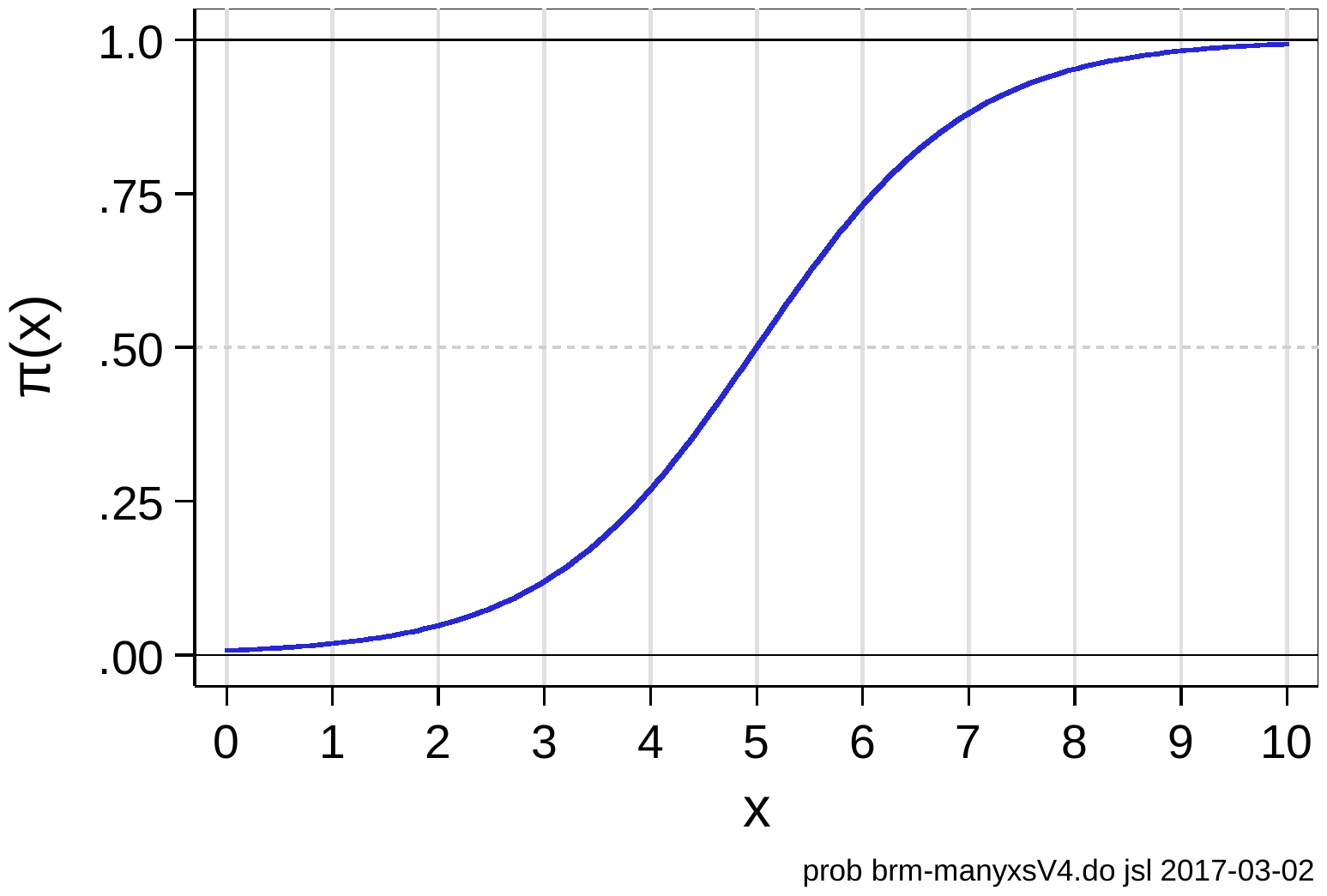
Model coefficients from the probability model are linear in the log-odds
In the probability metric, they are nonlinear, and constrained between 0 and 1

An S-shaped logistic curve for the probability of y = 1, rising from near 0 at x = 0 through 0.5 at x = 5 to near 1 at x = 10.

A latent variable model

The same model can be derived assuming a underlying latent continuum for the DV
- The unobserved propensity y* generates the observed y

A latent y-star line from minus infinity to infinity split at the threshold tau: values below tau are Not Voting for Trump (y = 0); values above are Voting for Trump (y = 1).

y* is linked to the observed y:

\[y_{i} = \begin{cases} 1 & \text{if } y_{i}^{*} > \tau \\ 0 & \text{if } y_{i}^{*} \leq \tau \end{cases}\]

Not all individuals who were observed at y=1 are planning to vote for Trump with the same certainty or “propensity y* to vote for him”
- One person may be considering voting third party
- Another person may be absolutely certain in their choice
Near τ (tau) a tiny change in y* changes the value of y

Identification: the scale of y* cannot be estimated

The structural model regresses latent y* on x:

\[y^{*} = \alpha + \beta x + \varepsilon\]

Since both y* and ε are unobserved, we do not know their means or variances
- Must make assumptions
- These assumptions affect size of β
  - We cannot directly interpret the magnitude of the β’s since we don’t know the true metric

Can all binary outcomes be viewed as observed manifestations of an underlying latent variable?
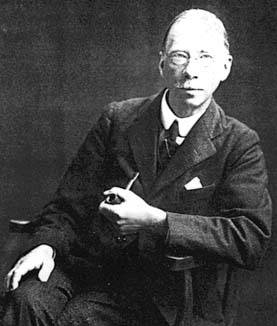
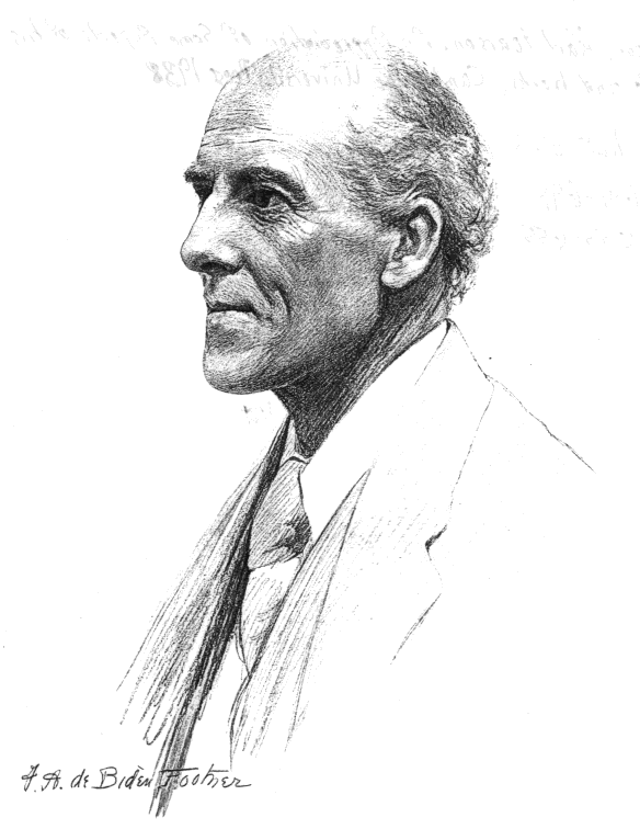
- George Udny Yule believed it was possible to define meaningful coefficients for 2x2 tables without assuming an underlying continuous distribution. Binary variables are inherently discrete
- Karl Pearson disagreed: “If Mr Yule’s views are accepted, irreparable damage will be done to the growth of modern statistical theory…” Yule’s ideas are “half-baked notions” and “specious reasoning”

Black-and-white portrait photograph of a man in a suit holding a pipe.

Does this debate matter for binary regression models?

The identical statistical model can be derived four ways:
- A latent variable model
- A probability model without a latent variable
- A generalized linear model (GLM)
- A random utility model (RUM) from economic theory*
Coefficient estimates are identical from each model

Pencil sketch portrait of an older man.

Gordon Ramsay meme: HEY KARL, SHUT IT.

*Not shown in these notes as it leads to an identical model; see Long (1997)