All graphs should have a descriptive, informative title
Both the x and y-axis should have a substantive label
General advice: talks vs articles
Font size
Talks: the font in the graph (titles, labels, axis titles, etc.) should be large enough to be easily read from afar
This is larger than you think!
Articles and Slides: the font size should flow seamlessly with the text of the article/slides*
Smaller, and the graph will be unreadable
Larger, and the graph will look out of place
Titles
Talks: a clear and descriptive title should be placed within the graph itself (usually at the top of the graph)
Articles: titles are generally typeset as part of the article—not as part of the graphics file itself, and are generally placed under the graph
*In R’s ggplot2, use base_size = #; in Stata, use scale(#) where # > 1 to increase all font sizes
Talks vs articles
“The clearest conclusion from most of these studies is that tables are best suited for looking up specific information, and graphs are better for perceiving trends and making comparisons and predictions… Subjects who indicated a preference for tables were generally novices: laypersons unused to statistical information or beginning college students. Studies using more sophisticated subjects showed a preference for graphs…” (Gelman, Pasarica, and Dodhia 2002)
Tables vs graphs
Talks: keep your audience awake (and aid more rapid interpretation): use graphics whenever possible
Articles: graphics are more effective for observing patterns and overall relationships; tables for specific numbers
I find graphics in the main text and tables in the Online Appendix useful
Always helpful to include the table (e.g., a regression table) somewhere just in case a reviewer or editor wants to see specifics (and, useful for meta-analyses)
General advice: fonts
Fonts within figures should present the information clearly and not distract from the important part of the figure: the data
Fonts for graphics should not be too “light” or too thin or they will be difficult to read – e.g., when there is a single number on an axis: 12345
They also should not be too “heavy” or compressed, or text can run together: 12345
Note that letters can look very different than numbers for some fonts: ABCabc 12345 (Georgia font)
Serif and sans serif fonts
I often see recommendations for sans serif fonts with the rationale they are more accessible; this is largely a myth (APA Style Guide)
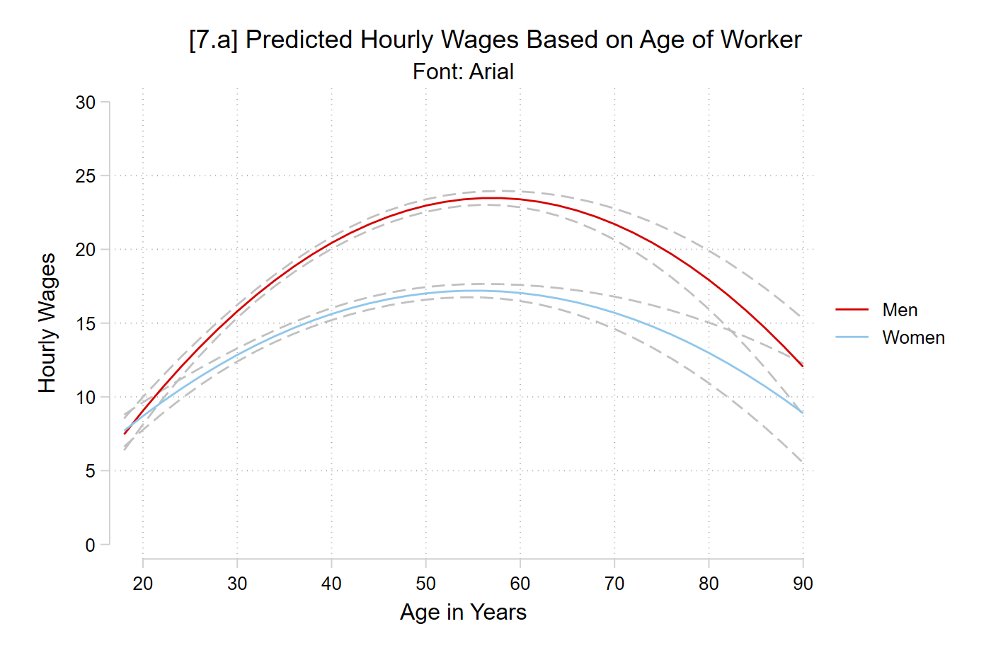
quiregress wages c.age##c.age##i.woman i.college i.racequi margins, at(age=(18(2)90) woman=(0 1))// 7.a - Arialgraphsetwindow fontface "Arial"marginsplot, plotopts(msym(none)) xlab(20(10)90) ylab(0(5)30) /// recastci(rline) ciopts(lpat(dash) col(gs12)) ///ytitle("Hourly Wages") xtitle("Age in Years") ///title("[7.a] Predicted Hourly Wages Based on Age of Worker", size(medium))///subtitle("Font: Arial")
Variables that uniquely identify margins: age woman
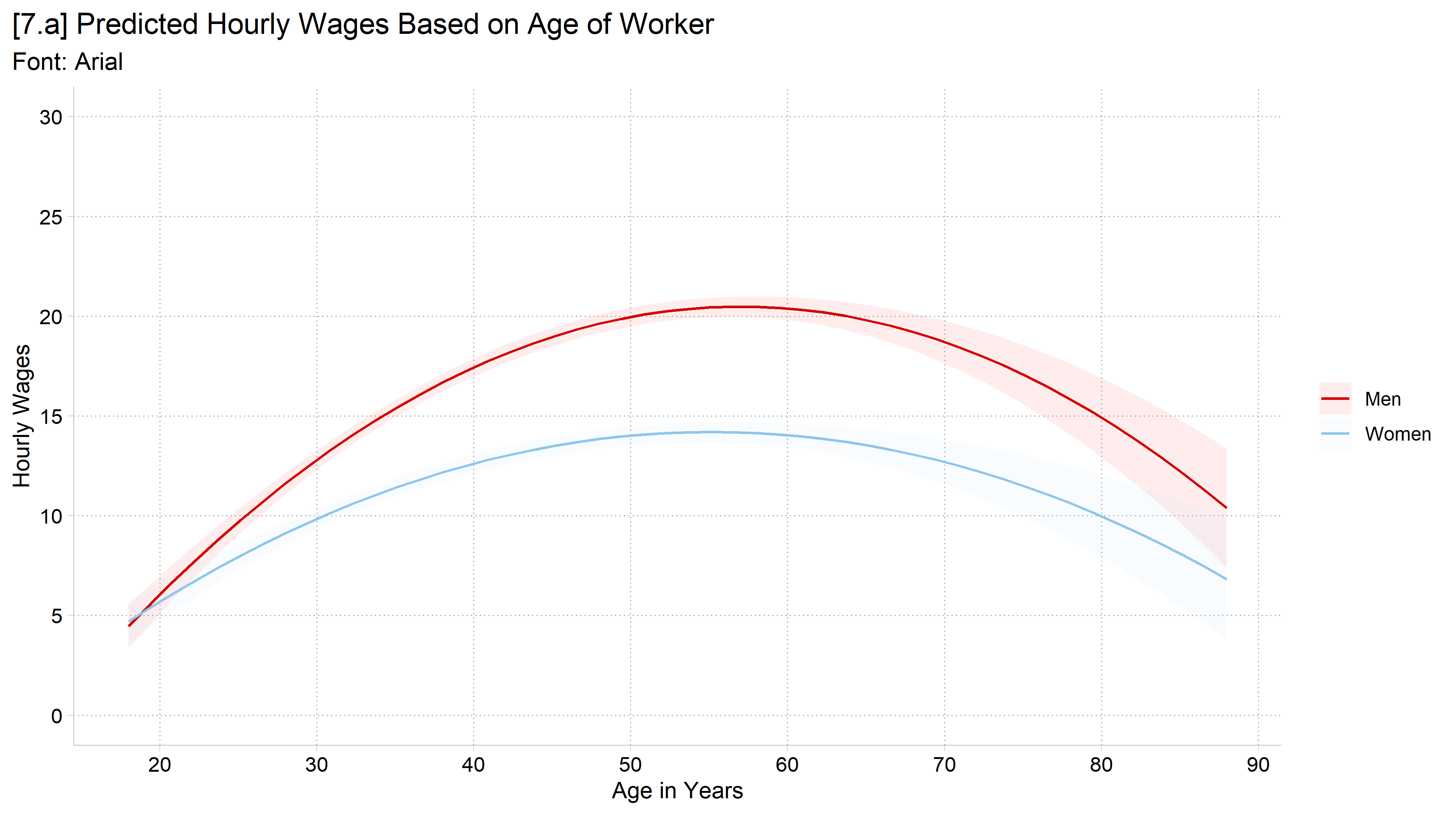
library(foreign) # load Stata datasetslibrary(ggplot2) # main graphics packagelibrary(dplyr) # data manipulation toolslibrary(marginaleffects) # predictions and marginal effectslibrary(cleanplots) # Mize's graphics scheme## Use cleanplots colors, markers, lines, and theme for all graphs ##cleanplots_defaults()theme_update(plot.title.position ="plot") # titles start at left edge of graph# General Social Survey Datagss <-droplevels(read.dta("https://tdmize.github.io/data/data/gss.dta"))# Ex graph for font and theme examplesgss_emp <-droplevels(filter(gss, year >=2000, employed ==1))wage_int <-lm(wages ~poly(age, 2, raw =TRUE) * woman + college + race, data = gss_emp)fig7 <-plot_predictions(wage_int, condition =c("age", "woman")) +labs(x ="Age in Years", y ="Hourly Wages", color ="", fill ="",title ="[7.#] Predicted Hourly Wages Based on Age of Worker") +scale_x_continuous(breaks =seq(20, 90, 10)) +scale_y_continuous(breaks =seq(0, 30, 5)) +coord_cartesian(ylim =c(0, 30))# 7.a - Arialfig7 +theme(text =element_text(family ="Arial")) +labs(title ="[7.a] Predicted Hourly Wages Based on Age of Worker",subtitle ="Font: Arial")
*Arial (or Helvetica – of which it is a clone) looks nice – but very “default”
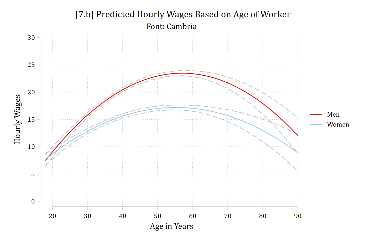
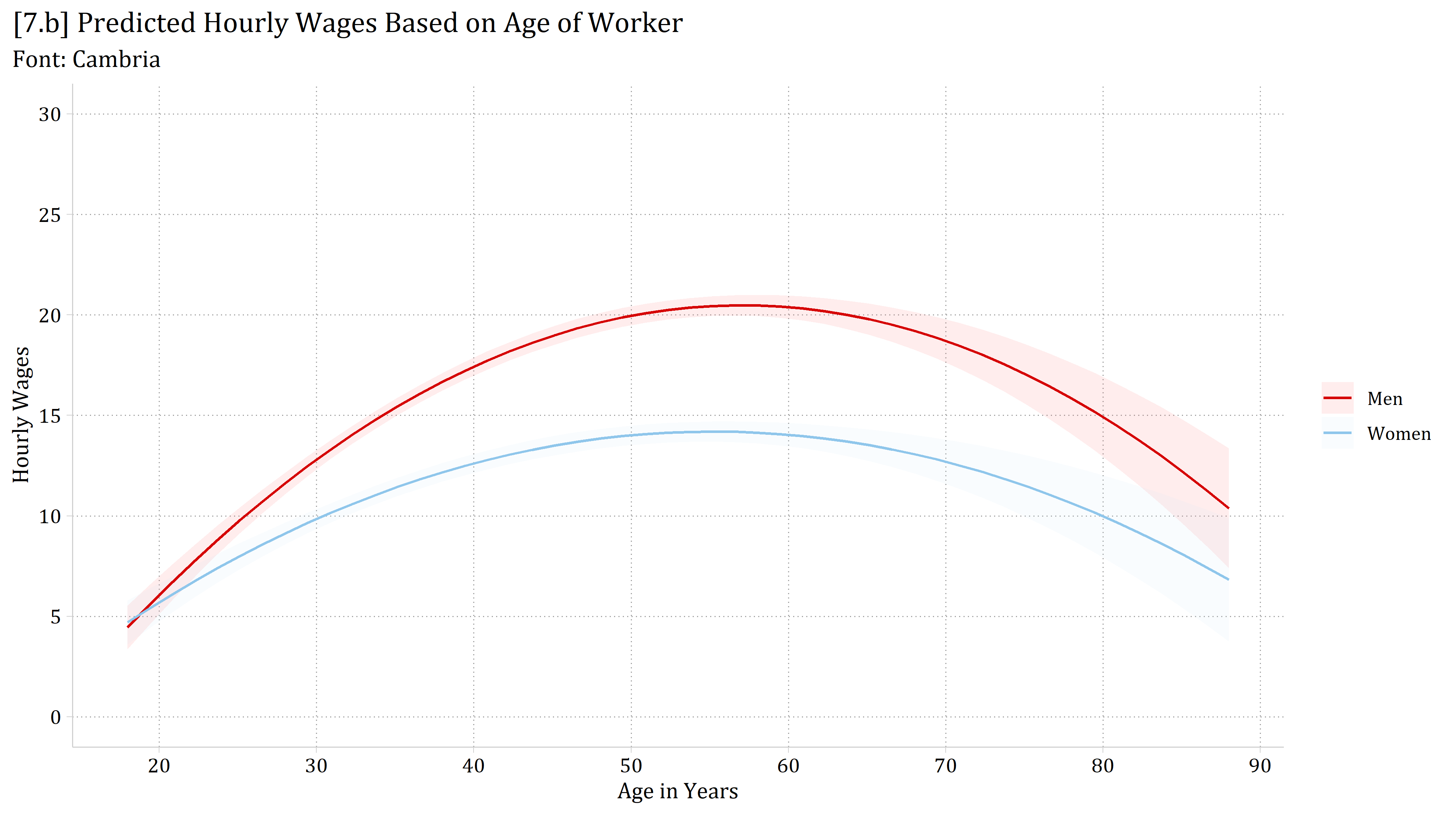
// 7.b - Cambriagraphsetwindow fontface "Cambria"marginsplot, plotopts(msym(none)) xlab(20(10)90) ylab(0(5)30) /// recastci(rline) ciopts(lpat(dash) col(gs12)) ///ytitle("Hourly Wages") xtitle("Age in Years") ///title("[7.b] Predicted Hourly Wages Based on Age of Worker", size(medium))///subtitle("Font: Cambria")
Variables that uniquely identify margins: age woman
# 7.b - Cambriafig7 +theme(text =element_text(family ="Cambria")) +labs(title ="[7.b] Predicted Hourly Wages Based on Age of Worker",subtitle ="Font: Cambria")
*Cambria is my normal go-to font for slides and graphics
In Stata, graph set changes the font for all later graphs. To go back to Stata’s default: graph set window fontface default
Graphics schemes in Stata
Stata’s graphics unfairly have a bad reputation
Stata’s graphical capabilities are impressive and flexible
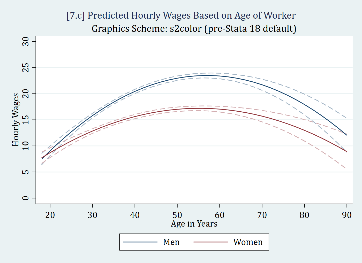
Stata’s default graphics choices (pre-Stata 18) were not great
Stata has many graphics schemes other than its pre-18 default (s2color)
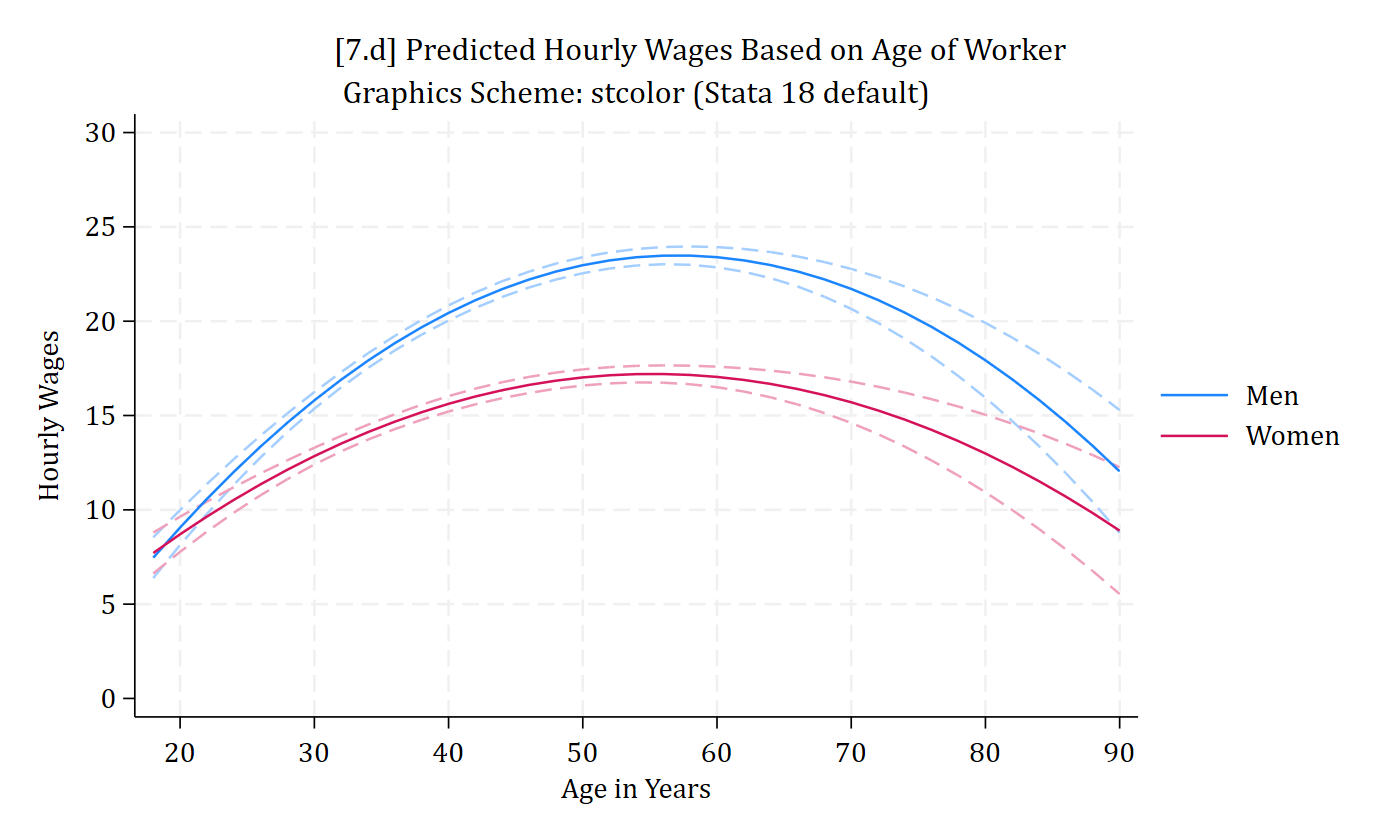
Stata 18’s default scheme (stcolor) is much better
// 7.d - stcolor (Stata 18 default)marginsplot, plotopts(msym(none)) xlab(20(10)90) ylab(0(5)30) /// recastci(rline) ciopts(lpat(dash) col(*.4)) ///ytitle("Hourly Wages") xtitle("Age in Years") ///title("[7.d] Predicted Hourly Wages Based on Age of Worker", size(medium))///subtitle("Graphics Scheme: stcolor (Stata 18 default)") scheme(stcolor)
Variables that uniquely identify margins: age woman
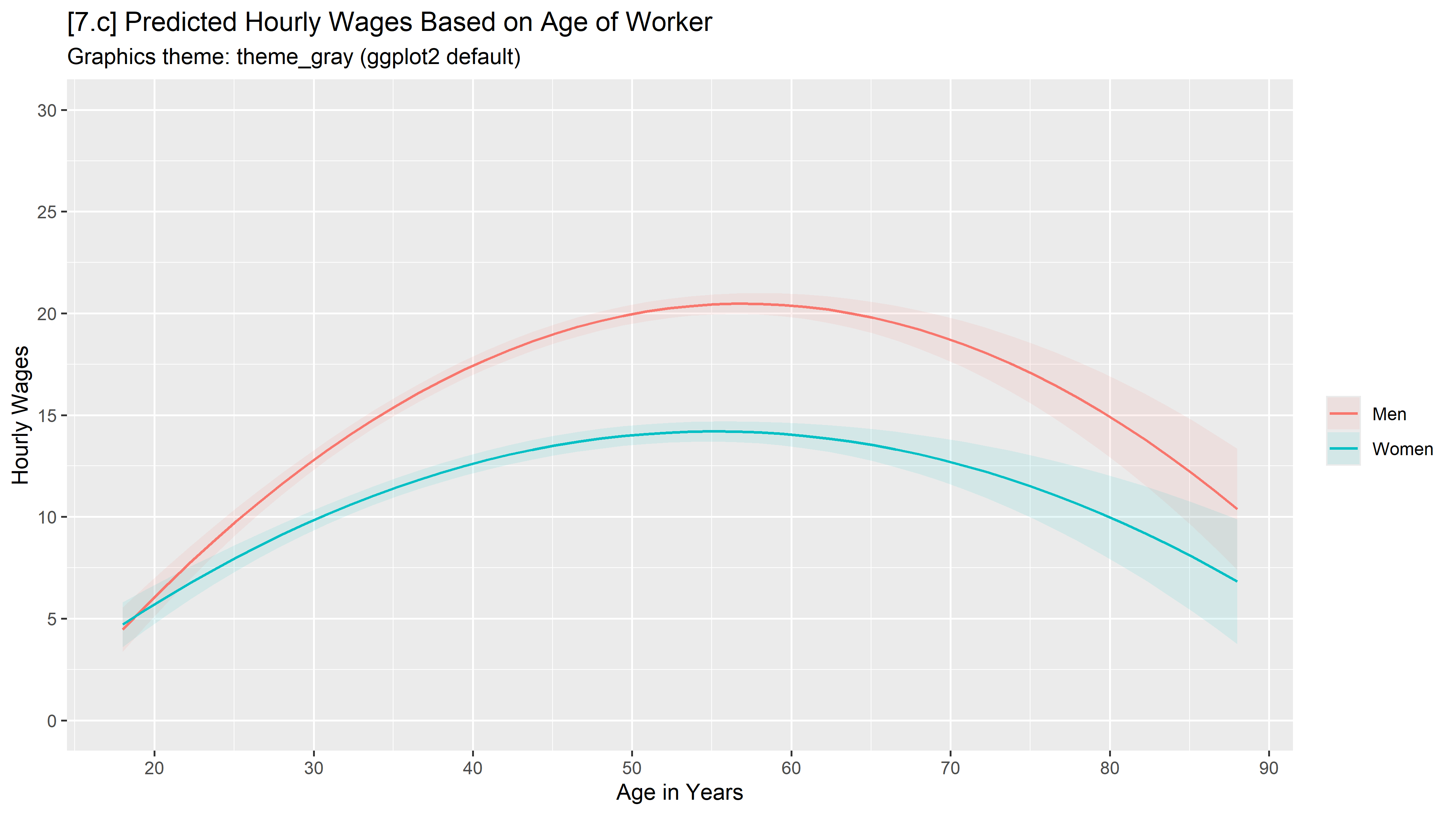
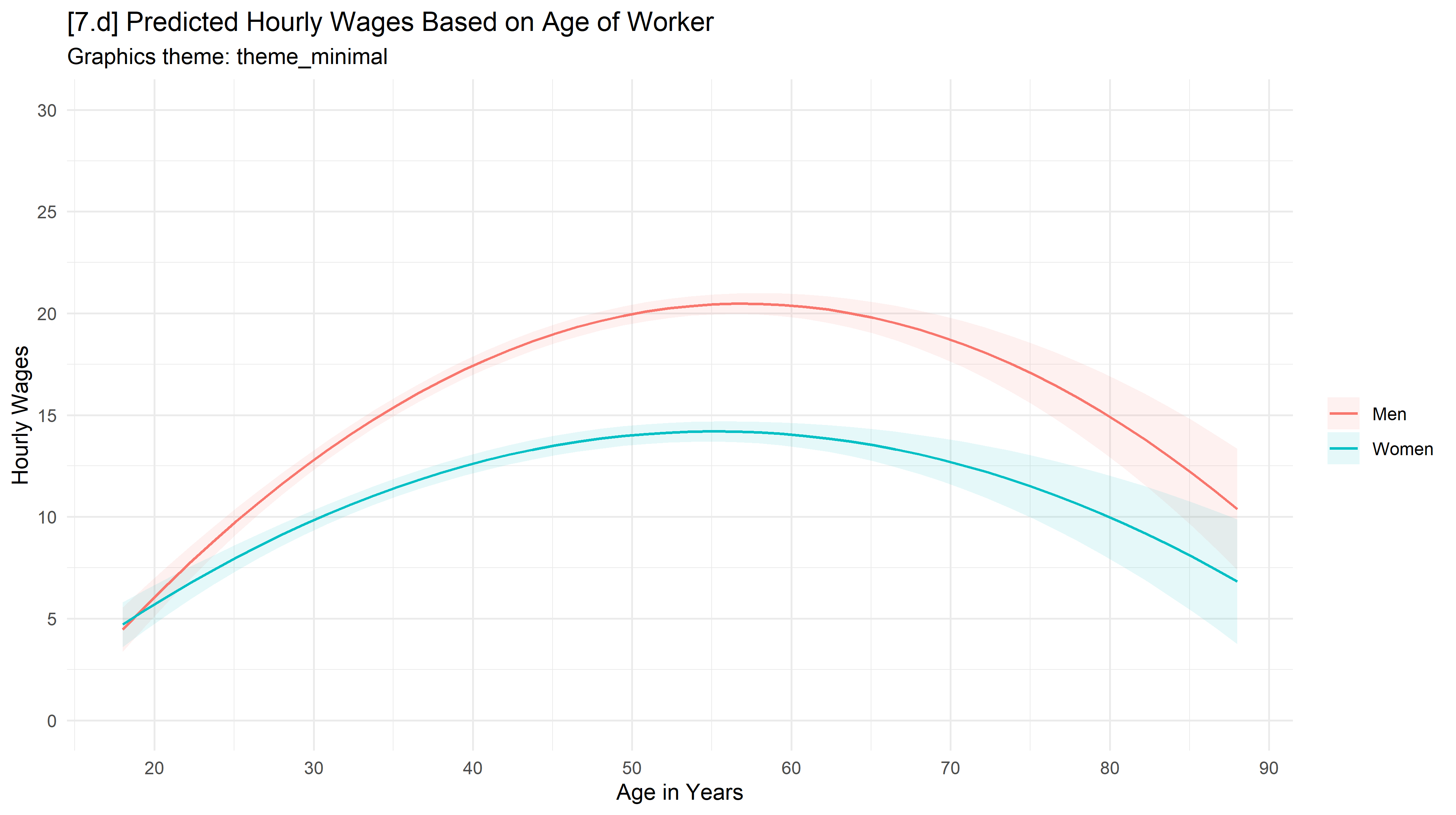
# 7.d - theme_minimalfig7 +theme_minimal() +scale_color_hue() +scale_fill_hue() +labs(title ="[7.d] Predicted Hourly Wages Based on Age of Worker",subtitle ="Graphics theme: theme_minimal")
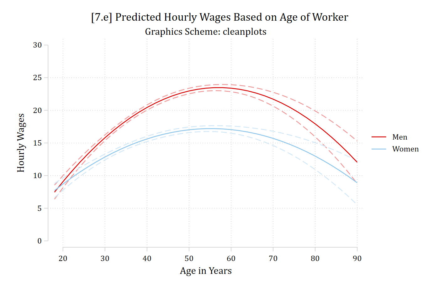
// 7.e - cleanplotsmarginsplot, plotopts(msym(none)) xlab(20(10)90) ylab(0(5)30) /// recastci(rline) ciopts(lpat(dash) col(*.4)) ///ytitle("Hourly Wages") xtitle("Age in Years") ///title("[7.e] Predicted Hourly Wages Based on Age of Worker", size(medium))///subtitle("Graphics Scheme: cleanplots") scheme(cleanplots)
Variables that uniquely identify margins: age woman
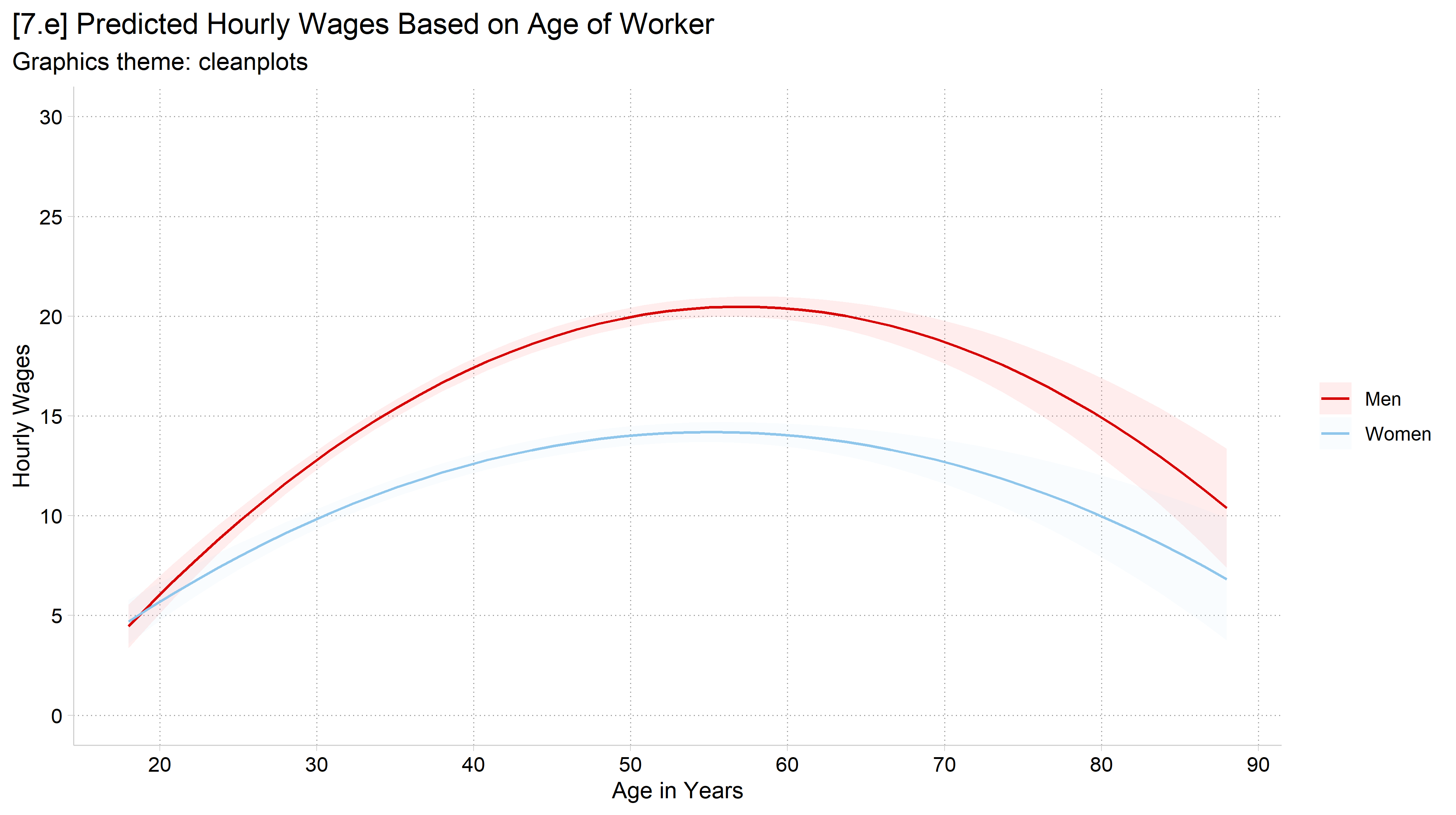
# 7.e - cleanplots (the default after cleanplots_defaults())fig7 +labs(title ="[7.e] Predicted Hourly Wages Based on Age of Worker",subtitle ="Graphics theme: cleanplots")
General advice: graphics file formats
I generally recommend PNG files
PNG works well across platforms (Word, PowerPoint, websites; Windows, Mac; etc.)
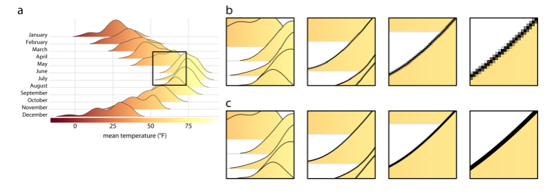
Avoid JPEG: JPEGs are optimized for photographs, not graphs
Vector graphics formats—PDF, EPS, and EMF—have some advantages but also some disadvantages
Advantage: they rescale without pixelating
Disadvantage: they are redrawn each time they are opened, so can look different across platforms (e.g., the original font may not be available)