2.4 Nonlinear Interaction Effects
- Things get complicated quickly when we combine interaction effects with nonlinearities
- When we get to models for categorical DVs, these are inherently nonlinear and interactive
- Linear regression models can be nonlinear and interactive
- From the examples above, we already know that: (a) age has a nonlinear effect (age2 coefficient was significant), and that (b) age has a different effect for men and women (age X woman product term coefficient is significant)
- Note (below) that to correctly model the nonlinear interaction effect you need five coefficients: age, age2, woman, woman*age, and woman*age2
- All five coefficients are necessary to properly estimate the nonlinear interaction effect
The limits of coefficients
use "https://tdmize.github.io/data/data/cda_gss", clear(cda_gss.dta | GSS 1972-2021 CDA - Categorical Data Analysis | date created 202
> 3)regress occprest c.age##c.age##i.woman i.college Source | SS df MS Number of obs = 58,304
-------------+---------------------------------- F(6, 58297) = 3180.18
Model | 2807908.65 6 467984.775 Prob > F = 0.0000
Residual | 8578800.25 58,297 147.156805 R-squared = 0.2466
-------------+---------------------------------- Adj R-squared = 0.2465
Total | 11386708.9 58,303 195.302281 Root MSE = 12.131
-------------------------------------------------------------------------------
occprest | Coefficient Std. err. t P>|t| [95% conf. interval]
--------------+----------------------------------------------------------------
age | 0.328 0.025 13.187 0.000 0.279 0.377
|
c.age#c.age | -0.003 0.000 -10.458 0.000 -0.003 -0.002
|
woman |
Women | 3.116 0.774 4.027 0.000 1.600 4.633
|
woman#c.age |
Women | -0.095 0.033 -2.831 0.005 -0.160 -0.029
|
woman#c.age#|
c.age |
Women | 0.000 0.000 1.359 0.174 -0.000 0.001
|
college |
College De.. | 16.216 0.121 134.015 0.000 15.979 16.453
_cons | 29.749 0.568 52.352 0.000 28.635 30.862
-------------------------------------------------------------------------------est store opintnlmod
est table opintnlmod, ///
title("[2.4.a] Occupational prestige linear regression model" ///
"Nonlinear interaction effects") ///
b(%5.3f) star(.05 .01 .001)[2.4.a] Occupational prestige linear regression model Nonlinear interaction
effects
---------------------------
Variable | opintnlmod
-------------+-------------
age | 0.328***
|
c.age#c.age | -0.003***
|
woman |
Women | 3.116***
|
woman#c.age |
Women | -0.095**
|
woman#c.age#|
c.age |
Women | 0.000
|
college |
College D.. | 16.216***
_cons | 29.749***
---------------------------
Legend: * p<.05; ** p<.01; *** p<.001¯\_(ツ)_/¯
qui margins, at(age=(20(5)80) woman=(0 1))
marginsplot, ///
    title("[2.4.b] Predicted Occupational Prestige Based on Person's Age and G
ender", size(medium)) ///
    subtitle("Interactive and Nonlinear Effect") ///
    ytitle("Occupational Prestige") ///
    recastci(rline) ciopts(lpat(dash) col(gs14)) ylab(38(2)46)
Variables that uniquely identify margins: age woman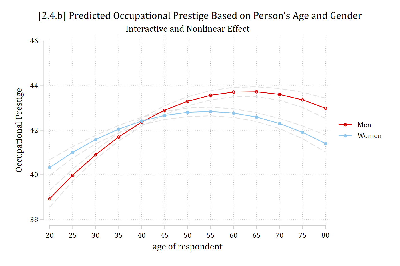
Now, the effect of age depends both on the value of age considered and based on whether the prediction is for a man or a woman
Interpreting nonlinear interaction effects with MEs
- It is best to provide examples and interpretations that best answer your research question
- Let’s say we are writing an article on the transition into early adulthood, thus we are mainly interested in the effect of age for those in their twenties
- Remember the effect will be different for men and women, so need to calculate an ME for men and an ME for women
- Let’s say we are writing an article on the transition into early adulthood, thus we are mainly interested in the effect of age for those in their twenties
mecompare age, start(age=20) covariates(woman=0) amount(10) models(opintnlmod)Predicting: Linear prediction
Marginal effects (N_opintnlmod=58304)
| ME # Estimate SE P>|z|
---------------------------------+---------------------------------------
age + 10 (centered) |
opintnlmod | 1 2.238 0.152 0.000mecompare age, start(age=20) covariates(woman=1) amount(10) models(opintnlmod)Predicting: Linear prediction
Marginal effects (N_opintnlmod=58304)
| ME # Estimate SE P>|z|
---------------------------------+---------------------------------------
age + 10 (centered) |
opintnlmod | 1 1.471 0.139 0.000A 10-year increase in age for 20-year-old men leads to about 2 points higher job prestige on average. For women, the same increase in age leads to about 1.26 points higher job prestige.
OR
On average, 30-year-old men are predicted to hold jobs that are about 2 points higher in job prestige than those held by 20-year-old men. 30-year-old women’s job prestige is higher than 20-year-old women’s by 1.26 points.
*See Appendix A2.5 for more on how to calculate these MEs
Equality of marginal effects: second differences
- Sometimes (depending on pattern of nonlinearities), can still be interesting / useful to examine if the effect, on average, differs across groups
- Does aging, on average, have a different effect for men and women?
- The test of the equality of MEs (sometimes called 1st differences) is called a 2nd difference
- Does aging, on average, have a different effect for men and women?
est restore opintnlmod(results opintnlmod are active now)mecompare age, by(woman) amount(sd)Predicting: Linear prediction
Marginal effects (N_m1=58304)
| ME # Estimate SE P>|z|
---------------------------------+---------------------------------------
age + SD (centered) |
Men | 1 1.503 0.080 0.000
Women | 2 0.591 0.074 0.000metest 2 - 1 | estimate se pvalue
---------------------------------+--------------------------------
age_woman_1 - age_woman_0 | -0.912 0.109 0.000 On average, a standard deviation increase in age for men is associated with a 1.50 point increase in occupational prestige. For women, aging shows a smaller, but still significant increase in job prestige (ME+SD | woman = 1 = 0.59; 2nd difference p < .001).
A caution about overlapping CIs
- An important (and often overlooked) part of interaction effects is the marginal effect of the secondary variable. E.g., The interpretations above focus on the effect of age—gender is a secondary consideration. However, what about the effect of gender? There is an interesting story there too
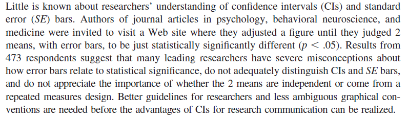
- Importantly, when confidence intervals do not overlap this indicates that the group difference (i.e., men vs women in our plot) is significant. When the confidence interval does overlap this may or may not indicate the group difference is non-significant*: you must test for this directly. As Belia et al. (2005) gently put it:
*NOTE: These general rules are only true for independent non-overlapping samples. It is even more complicated with clustered data (e.g., multilevel or longitudinal data)
Visualizing significant group differences
- Fortunately, there are fairly straightforward ways to calculate and visualize significance information for group differences
- The first method I recommend is to calculate and then plot the marginal effect of the binary/nominal IV across the range of the continuous IV (here, the ME of gender across the range of age)
- Go back to the last graph. What is the ME of gender? It is simply the gap between the red and blue lines. That shows you the difference between men and women at each age
- Compare the last graph to the one below
est restore opintnlmod(results opintnlmod are active now)qui margins, dydx(woman) at(age=(20(5)80))
marginsplot, ///
recastci(rline) ciopts(lpat(dash) col(gs14)) yline(0) ylab(-2(1)2) ///
title("[2.4.c] Marginal Effect of Gender across Range of Age", size(medlar
ge)) ///
subtitle("Effects above zero indicate women have higher job prestige") ///
ytitle("Effect of Gender: Women - Men")Variables that uniquely identify margins: age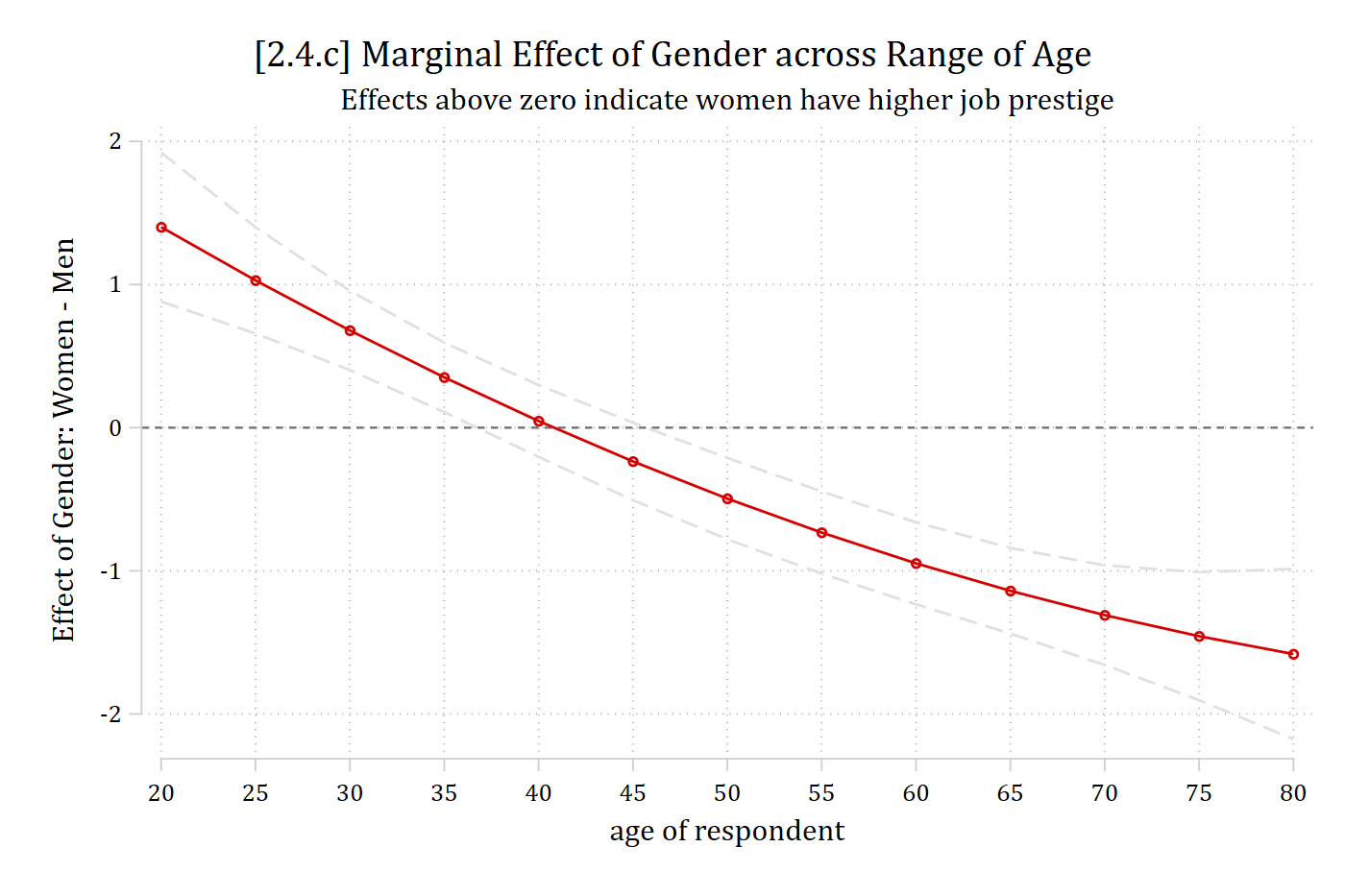
*This is a direct test of the effect of gender: whenever the confidence interval overlaps zero = no significant group difference (see interpretation below)
Example interpretation of the plot above
As Figure # shows, at younger ages, women have higher occupational prestige than men (from age 20 to about age 37). From ages 37 to 45, men and women have similar occupational prestige scores. A gender gap reappears after age 45; however, at these older ages, the gender gap reverses, with men having higher occupational prestige than do women.
To see at exactly what ages the group difference is or is not significant:
mtable, dydx(woman) at(age=(20(1)80)) stat(est se p)Expression: Linear prediction, predict()
| age d xb se p
----------+---------------------------------------
1 | 20 1.401 0.265 0.000
2 | 21 1.325 0.248 0.000
3 | 22 1.250 0.232 0.000
4 | 23 1.175 0.217 0.000
5 | 24 1.102 0.202 0.000
6 | 25 1.029 0.189 0.000
7 | 26 0.957 0.177 0.000
8 | 27 0.886 0.166 0.000
9 | 28 0.816 0.157 0.000
10 | 29 0.747 0.148 0.000
11 | 30 0.679 0.141 0.000
12 | 31 0.612 0.135 0.000
13 | 32 0.545 0.131 0.000
14 | 33 0.480 0.127 0.000
15 | 34 0.415 0.125 0.001
16 | 35 0.352 0.124 0.005
17 | 36 0.289 0.123 0.019
18 | 37 0.227 0.124 0.067
19 | 38 0.166 0.125 0.183
20 | 39 0.106 0.126 0.401
21 | 40 0.047 0.128 0.714
22 | 41 -0.011 0.130 0.930
23 | 42 -0.069 0.132 0.602
24 | 43 -0.125 0.134 0.350
25 | 44 -0.181 0.136 0.184
26 | 45 -0.235 0.138 0.088
27 | 46 -0.289 0.140 0.039
28 | 47 -0.342 0.141 0.016
29 | 48 -0.394 0.143 0.006
30 | 49 -0.445 0.144 0.002
31 | 50 -0.495 0.145 0.001
32 | 51 -0.545 0.146 0.000
33 | 52 -0.593 0.146 0.000
34 | 53 -0.640 0.146 0.000
35 | 54 -0.687 0.146 0.000
36 | 55 -0.733 0.146 0.000
37 | 56 -0.777 0.146 0.000
38 | 57 -0.821 0.146 0.000
39 | 58 -0.864 0.146 0.000
40 | 59 -0.906 0.146 0.000
41 | 60 -0.947 0.146 0.000
42 | 61 -0.988 0.147 0.000
43 | 62 -1.027 0.147 0.000
44 | 63 -1.065 0.149 0.000
45 | 64 -1.103 0.150 0.000
46 | 65 -1.139 0.153 0.000
47 | 66 -1.175 0.156 0.000
48 | 67 -1.210 0.160 0.000
49 | 68 -1.244 0.165 0.000
50 | 69 -1.277 0.171 0.000
51 | 70 -1.309 0.178 0.000
52 | 71 -1.340 0.186 0.000
53 | 72 -1.371 0.195 0.000
54 | 73 -1.400 0.205 0.000
55 | 74 -1.429 0.216 0.000
56 | 75 -1.456 0.228 0.000
57 | 76 -1.483 0.241 0.000
58 | 77 -1.509 0.255 0.000
59 | 78 -1.534 0.270 0.000
60 | 79 -1.558 0.286 0.000
61 | 80 -1.581 0.303 0.000
Specified values where .n indicates no values specified with at()
| No at()
----------+---------
Current | .nPresenting nonlinear interaction effects
- I would always include the plot of predictions in an article for a nonlinear interaction effect (figure 2.4.b above)
- These are familiar to readers and easily understood
- The graph of MEs (2.4.c above) is harder to understand, especially out of context
- I usually present these second in my article; when possible, alongside the graph of predictions (see below)
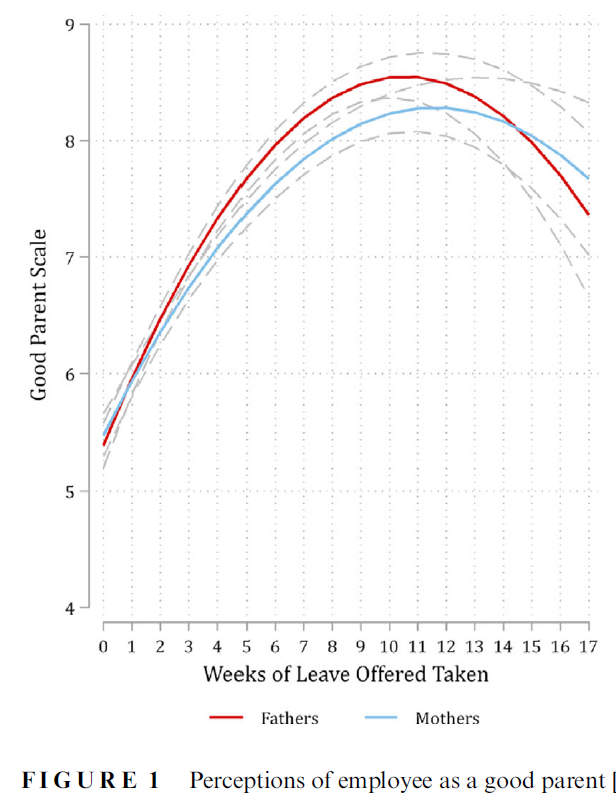
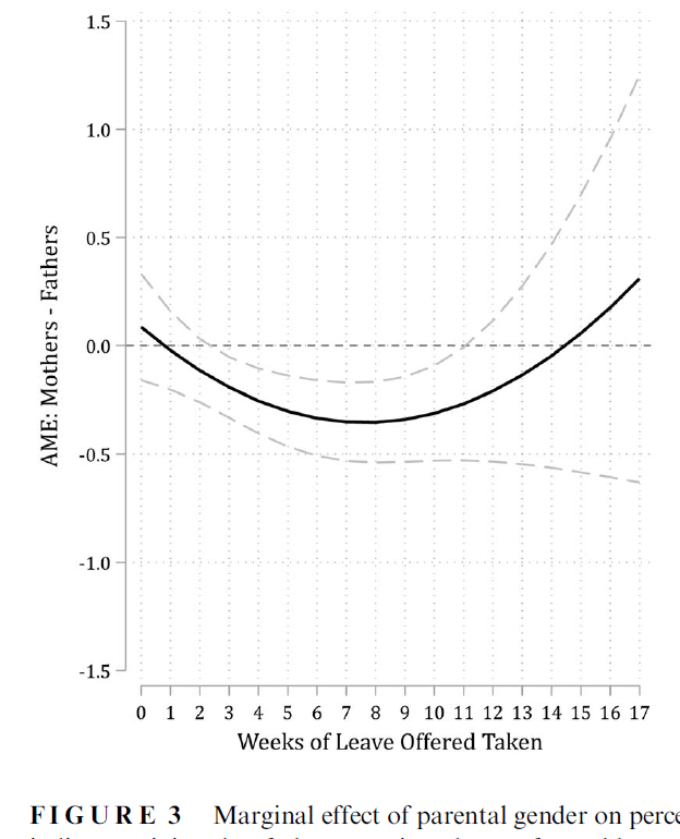
*I like including both graphs in a single paper (often as separate panels) to help the reader follow what the second graph shows. Example from Petts, Kaufman, and Mize 2023
Example write-up of occupational prestige findings
est restore opintnlmod(results opintnlmod are active now)mecompare age woman, amount(sd) models(opintnlmod)Predicting: Linear prediction
Marginal effects (N_opintnlmod=58304)
| ME # Estimate SE P>|z|
---------------------------------+---------------------------------------
age + SD (centered) |
opintnlmod | 1 1.013 0.054 0.000
---------------------------------+---------------------------------------
woman |
Women - Men |
opintnlmod | 2 -0.165 0.101 0.101Overall, individuals tend to hold more prestigious jobs when they are older compared to when they were younger—but the relationship is nonlinear. On average, a standard deviation increase in age (about 17.2 years) is associated with a 1.01 increase in occupational prestige (p < 0.001). However, Figure # illustrates the nonlinearities: aging is associated with increased occupational prestige until the late 50s, but the effect then reverses, with aging associated with lower occupational prestige late in life. In addition to the nonlinear effect of age, there are important differences in the effect of age based on a person’s gender. Women have higher occupational prestige than men from age 20 to about 37, but the effect then reverses, with men having higher occupational prestige after the age of about 45. Overall, aging shows a stronger association for men than women (2nd diff p < .001).