4.0 Nominal DVs

German Election 2021.

Preliminary results of the 2021 German election (percent of votes): SPD 25.7, CDU/CSU 24.1, Greens 14.8, FDP 11.5, AfD 10.3, The Left 4.9, others 6.1.

Level of measurement

“measurement…is defined as the assignment of numerals to objects or events according to rules.” (Stevens 1946)

  • S.S. Stevens (1946) introduced terms nominal and ordinal
    • Nominal scales have numbers assigned to categories as labels with no ordering implied by the numbers
    • Ordinal scales have numbers indicating rank ordering on one attribute
  • Hotly debated and critiqued when it was proposed, his taxonomy is now firmly established
  • Ordinal models assume his definition of ordinal for the DV (and more)
  • Nominal models do not make assumptions about the relationship among categories of the DV*

*But see the discussion of the IIA assumption at end of these notes (4.6)

The bias-efficiency trade-off

regress y x1 x2 x3      // true model
regress y x1            // bias
regress y x1 x2 x3 x4   // inefficiency

Effects of assuming wrong level of measurement

Model choice (assumed level of DV for analysis) True level of DV: Nominal Ordinal Continuous*
Nominal Ideal Inefficient Inefficient
Ordinal Biased Ideal Inefficient
Continuous Biased Biased Ideal

*I am not distinguishing between interval and ratio variables here

  • If outcome is ordinal and model is nominal, it is inefficient, but often safe choice
    • The only way to be sure an ordinal model fits the data is to examine a nominal model for the same DV

Multinomial logit as an extension of binary logit

  • Example: Political views at different ages
    • Data: GSS 2016 – 2021

Binary Example #1:

DV: Identify as “conservative = 1” or “not conservative = 0”

IV: Age

Controls: Gender, race, education, family income, employment status, marital status, parental status

Binary Example #2:

DV: Identify as “not conservative = 1” or “conservative = 0”

IV: Age

Controls: Gender, race, education, family income, employment status, marital status, parental status

use "https://tdmize.github.io/data/data/cda_gss", clear
(cda_gss.dta |  GSS 1972-2021 CDA - Categorical Data Analysis | date created 202
> 3)
keep if year >= 2016 & year <= 2021
(59,599 observations deleted)
gen notconserv = conserv
(280 missing values generated)
lab var notconserv "Not Conservative"
recode notconserv 0=1 1=0
(8,967 changes made to notconserv)
lab def notlab 0"Conservative" 1"Not Conservative"
lab val notconserv notlab
drop if missing(conserv, age, woman, race3, college, married, parent, faminc)
(1,421 observations deleted)
*4.0.a Conservative = 1
qui logit conserv c.age i.woman i.race3 i.college ///
    i.married i.parent c.faminc i.employed
est store conmod
qui margins, at(age=(18(2)88)) saving(conmod, replace)
marginsplot, xlab(18(10)88) ylab(0(0.2)1) noci ///
    title("[4.0.a] Pr(Identifying as Conservative)", size(medlarge)) ///
    text(.2 30 "Pr = 0.27" .3 70 "Pr = 0.38", color(red)) ///
    plotopts(msym(none)) saving(conserv, replace)
Variables that uniquely identify margins: age
(file conserv.gph not found)
file conserv.gph saved
*4.0.b Not Conservative = 1
qui logit notconserv c.age i.woman i.race3 i.college ///
    i.married i.parent c.faminc i.employed
est store notconmod
qui margins, at(age=(18(2)88)) saving(notconmod, replace)
marginsplot, xlab(18(10)88) ylab(0(0.2)1) noci ///
    title("[4.0.b] Pr(NOT Identifying as Conservative)", size(medlarge)) ///
    text(.8 30 "Pr = 0.73" .7 70 "Pr = 0.62", color(purple)) ///
    plotopts(msym(none) lcol(purple) lpat(dash)) saving(notcon, replace)
Variables that uniquely identify margins: age
(file notcon.gph not found)
file notcon.gph saved
graph combine conserv.gph notcon.gph, scale(1.1)

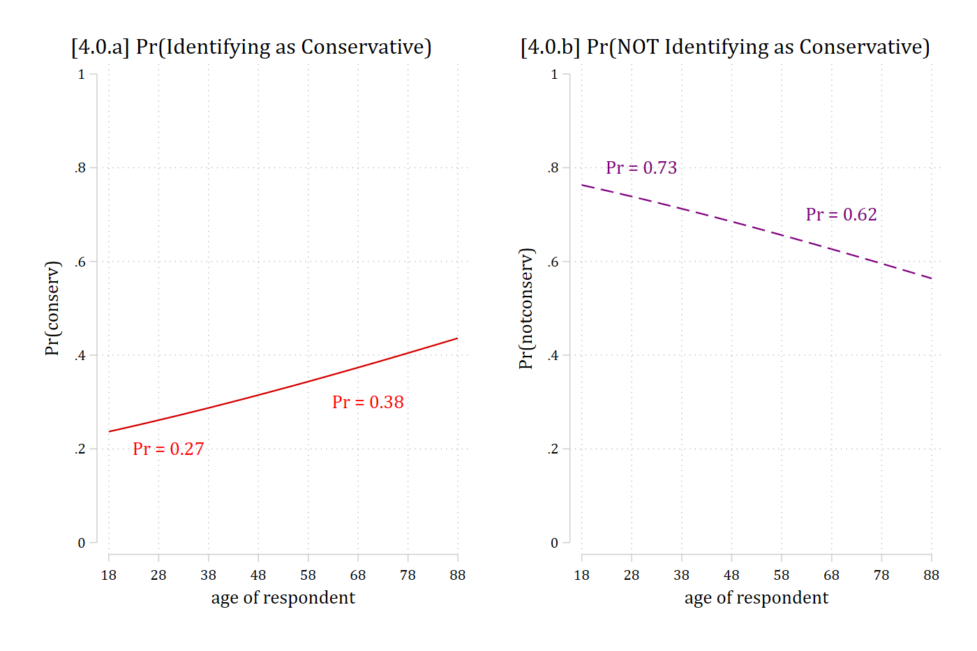
Two panels of predicted probabilities by age from 18 to 88: [4.0.a] Pr(conservative) rises from about 0.24 to 0.43 (0.27 at age 30, 0.38 at age 70); [4.0.b] Pr(not conservative) falls from about 0.76 to 0.57 (0.73 at 30, 0.62 at 70).

library(haven)           # import Stata data and labels
library(dplyr)           # data manipulation
library(ggplot2)         # graphs
library(nnet)            # multinomial logit: multinom()
library(marginaleffects) # predictions and marginal effects
library(cleanplots)      # graph scheme
cleanplots_defaults()

# Center changes in continuous IVs on each observation's value
options(marginaleffects_contrast_direction = "center")

gss <- read_dta("https://tdmize.github.io/data/data/cda_gss.dta")

gss <- gss |> filter(year >= 2016 & year <= 2021)

# Keep model variables; drop any missing data
gss <- gss[c("conserv", "polviews3", "age", "woman", "race3", "college",
  "married", "parent", "faminc", "employed")]
gss <- gss[complete.cases(gss[c("conserv", "age", "woman", "race3", "college",
  "married", "parent", "faminc")]), ]

# Not conservative = 1; treat binary/nominal variables as factors
gss <- gss |>
  mutate(notconserv = 1 - conserv,
    across(c(polviews3, woman, race3, college, married, parent, employed), as_factor)) |>
  droplevels()

# 4.0.a Conservative = 1
conmod <- glm(conserv ~ age + woman + race3 + college + married + parent +
  faminc + employed, data = gss, family = binomial(link = "logit"))

# 4.0.b Not Conservative = 1
notconmod <- glm(notconserv ~ age + woman + race3 + college + married + parent +
  faminc + employed, data = gss, family = binomial(link = "logit"))

# Predictions at ages 18 to 88 from each model
pr_age <- bind_rows(
  "[4.0.a] Pr(Identifying as Conservative)" = avg_predictions(conmod, by = "age",
    newdata = datagrid(age = seq(18, 88, 2), grid_type = "counterfactual")),
  "[4.0.b] Pr(NOT Identifying as Conservative)" = avg_predictions(notconmod, by = "age",
    newdata = datagrid(age = seq(18, 88, 2), grid_type = "counterfactual")),
  .id = "model")

pr_labels <- data.frame(model = rep(unique(pr_age$model), each = 2),
  age = c(30, 70, 30, 70), y = c(.2, .3, .8, .7),
  label = c("Pr = 0.27", "Pr = 0.38", "Pr = 0.73", "Pr = 0.62"))

ggplot(pr_age, aes(x = age, y = estimate, color = model, linetype = model)) +
  geom_line() +
  geom_text(data = pr_labels, aes(y = y, label = label), show.legend = FALSE) +
  facet_wrap(~ model) +
  scale_color_manual(values = c("red", "purple")) +
  scale_linetype_manual(values = c("solid", "dashed")) +
  scale_x_continuous(breaks = seq(18, 88, 10)) +
  scale_y_continuous(breaks = seq(0, 1, .2), limits = c(0, 1)) +
  labs(x = "age of respondent", y = "Pr(y = 1)") +
  theme(legend.position = "none")

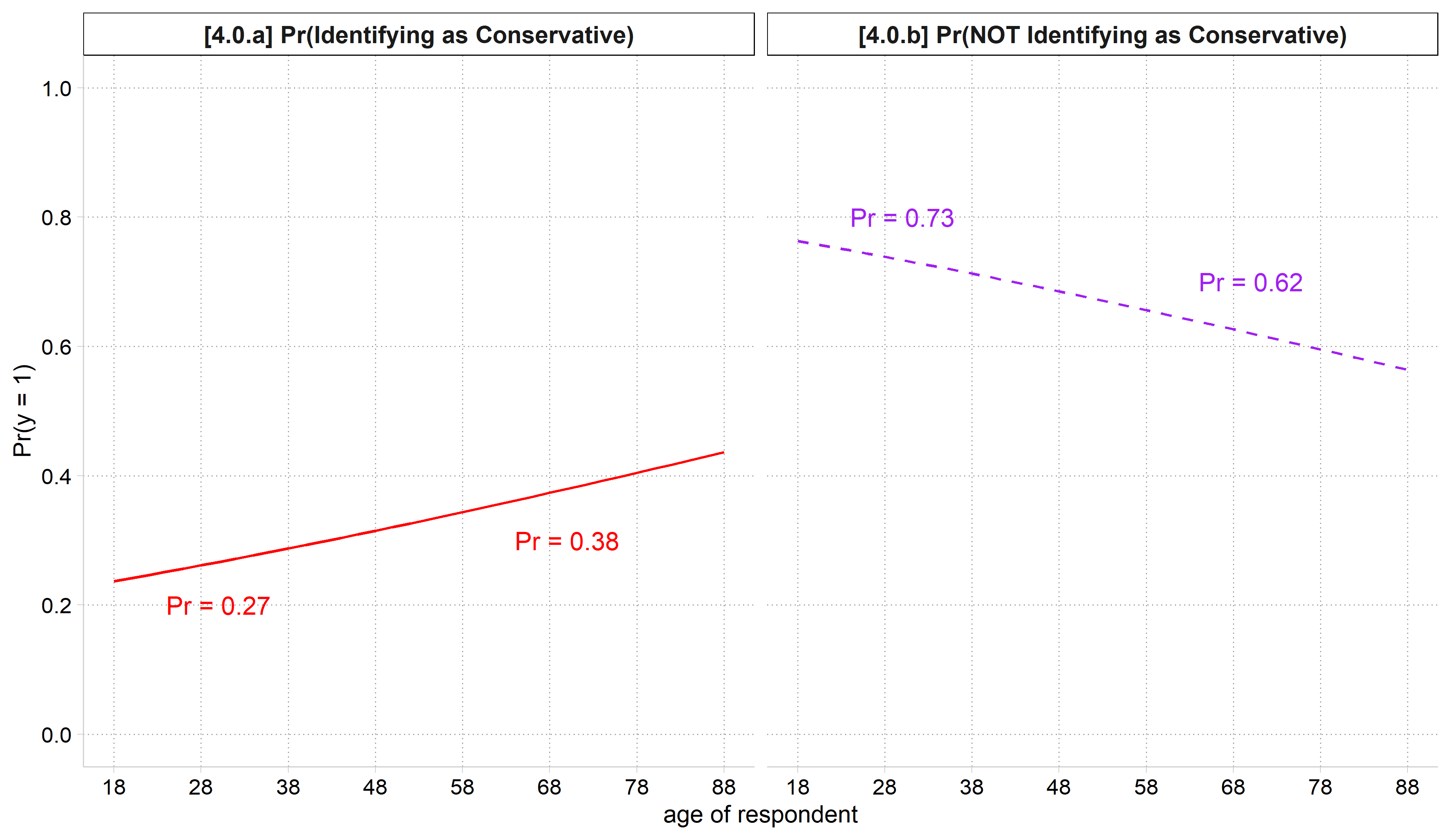
Two panels of predicted probabilities by age from 18 to 88: [4.0.a] Pr(conservative) rises from about 0.24 to 0.43 (0.27 at age 30, 0.38 at age 70); [4.0.b] Pr(not conservative) falls from about 0.76 to 0.57 (0.73 at 30, 0.62 at 70).

The models are identical. Choice of how to code DV is arbitrary*

*Good practice to code your binary DV in line with direction of your hypotheses

*4.0.c
combomarginsplot conmod notconmod, ///
    labels("Pr(Conservative)" "Pr(Not Conserv.)") noci ///
    file1opts(msym(none)) ///
    file2opts(msym(none) lcol(purple) lpat(dash)) ///
    xlab(18(10)88) ylab(0(0.2)1) ytitle("Pr(Conservative or Not)") ///
    title("[4.0.c] Pr(Identifying as Conservative or Not) 2016 - 2021", size(m
edlarge)) ///
    text(.2 30 "Pr = 0.27" .3 70 "Pr = 0.38", color(red)) ///
    text(.8 30 "Pr = 0.73" .7 70 "Pr = 0.62", color(purple))
  Variables that uniquely identify margins: age _filenumber

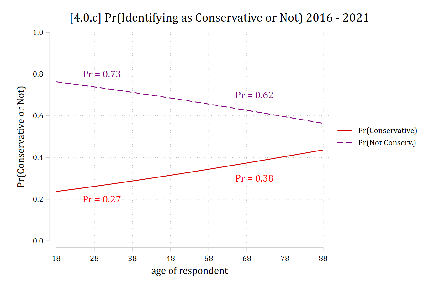
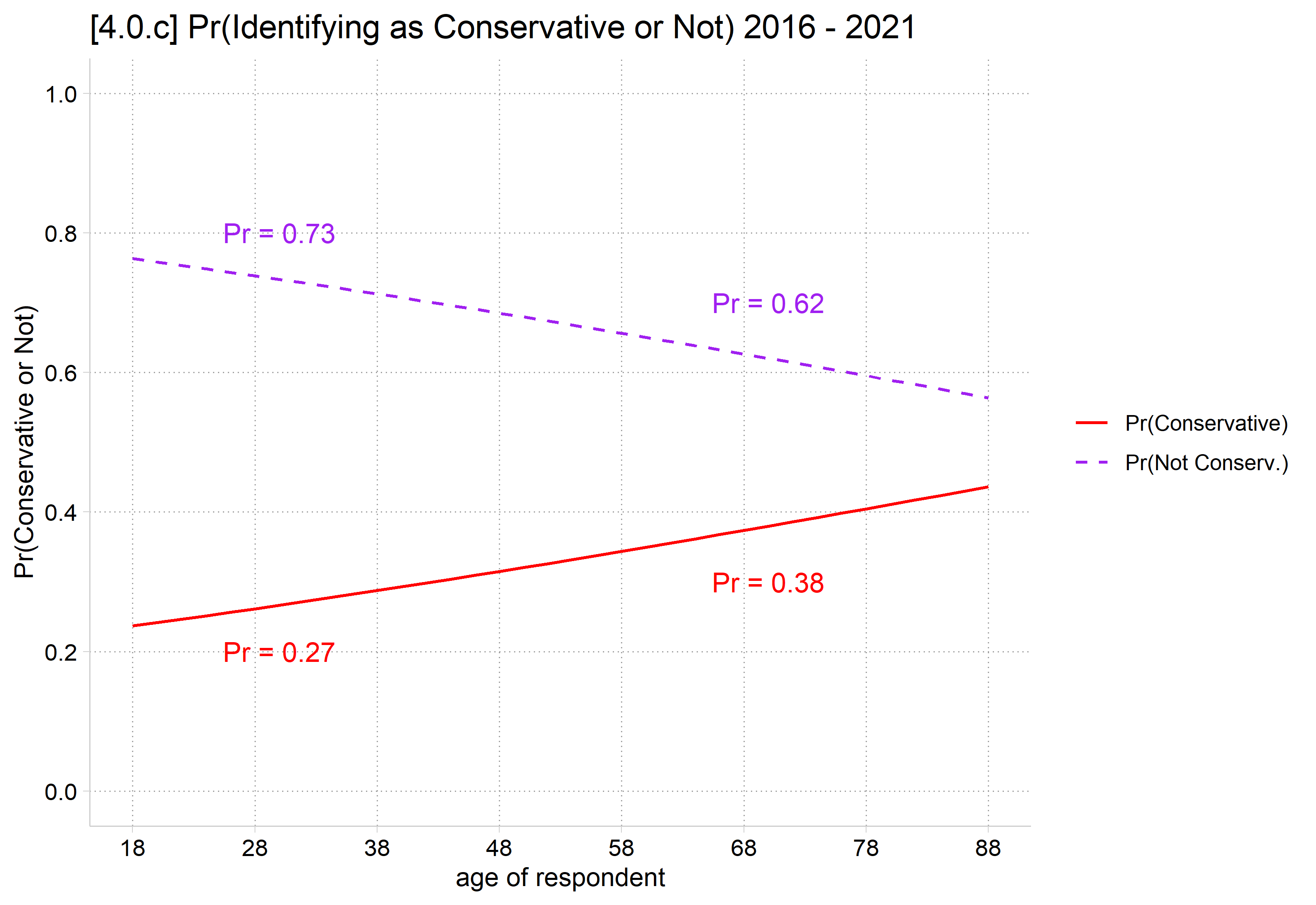
[4.0.c] Both lines on one graph by age: Pr(conservative) rises from about 0.24 to 0.43 and Pr(not conservative) falls from about 0.76 to 0.57; the two lines mirror each other around 0.5.

# 4.0.c
pr_age <- pr_age |>
  mutate(outcome = ifelse(model == unique(model)[1], "Pr(Conservative)", "Pr(Not Conserv.)"))

ggplot(pr_age, aes(x = age, y = estimate, color = outcome, linetype = outcome)) +
  geom_line() +
  annotate("text", x = c(30, 70), y = c(.2, .3), label = c("Pr = 0.27", "Pr = 0.38"),
    color = "red") +
  annotate("text", x = c(30, 70), y = c(.8, .7), label = c("Pr = 0.73", "Pr = 0.62"),
    color = "purple") +
  scale_color_manual(values = c("red", "purple")) +
  scale_linetype_manual(values = c("solid", "dashed")) +
  scale_x_continuous(breaks = seq(18, 88, 10)) +
  scale_y_continuous(breaks = seq(0, 1, .2), limits = c(0, 1)) +
  labs(title = "[4.0.c] Pr(Identifying as Conservative or Not) 2016 - 2021",
    x = "age of respondent", y = "Pr(Conservative or Not)", color = NULL, linetype = NULL)

[4.0.c] Both lines on one graph by age: Pr(conservative) rises from about 0.24 to 0.43 and Pr(not conservative) falls from about 0.76 to 0.57; the two lines mirror each other around 0.5.

We usually only plot Pr(y = 1) because Pr(y = 0) is redundant information

Average marginal effects in binary logit

*Conservative = 1
mecompare age, amount(sd) model(conmod)
Predicting: Pr(conserv)
Marginal effects (N_conmod=7823)

                                 |  ME #   Estimate         SE      P>|z|
---------------------------------+---------------------------------------
age + SD (centered)              |                                       
                          conmod |     1      0.049      0.006      0.000
*Not Conservative = 1
mecompare age, amount(sd) model(notconmod)
Predicting: Pr(notconserv)
Marginal effects (N_notconmod=7823)

                                 |  ME #   Estimate         SE      P>|z|
---------------------------------+---------------------------------------
age + SD (centered)              |                                       
                       notconmod |     1     -0.049      0.006      0.000
# Conservative = 1
avg_comparisons(conmod, variables = list(age = sd(gss$age)))

 Estimate Std. Error    z Pr(>|z|)    S 2.5 % 97.5 %
   0.0489    0.00606 8.06   <0.001 50.2 0.037 0.0607

Term: age
Type: response
Comparison: +17.3603297947298
# Not Conservative = 1
avg_comparisons(notconmod, variables = list(age = sd(gss$age)))

 Estimate Std. Error     z Pr(>|z|)    S   2.5 % 97.5 %
  -0.0489    0.00606 -8.06   <0.001 50.2 -0.0607 -0.037

Term: age
Type: response
Comparison: +17.3603297947298

Binary logit model with new notation

  • Usually we think of binary logit as modeling Pr(y = 1)
    • An equivalent way to present the model is the Pr(y = A) vs Pr(y = B)
      • A = 1 and B = 0
  • The logit model is linear in the logit for outcome A versus B

\[\ln\left[\frac{\Pr(y = A\,|\,\mathbf{x})}{\Pr(y = B\,|\,\mathbf{x})}\right] = \beta_{0,A|B} + \beta_{x_{1},A|B}\,x_{1,i} + \ldots + \beta_{x_{k},A|B}\,x_{k,i}\]

  • Exponentiated coefficients represent the multiplicative effect of a one-unit increase in xk on the odds of outcome A vs B
  • We can obtain predicted probabilities of category A and B with:

\[\Pr(y = A\,|\,\mathbf{x}) = \frac{\exp(\mathbf{x}_{i}\boldsymbol{\beta})}{1 + \exp(\mathbf{x}_{i}\boldsymbol{\beta})}\]

\[\Pr(y = B\,|\,\mathbf{x}) = 1 - \Pr(y = A\,|\,\mathbf{x})\]

Multinomial logit as an extension of binary logit

  • Multinomial logit is no more complicated than binary logit
    • The recommended methods of interpretation are the same:
      • Marginal effects (especially AMEs)
      • Plots of predicted probabilities
    • The limitations/problems with coefficients and odds ratios from binary logit apply equally to multinomial logit
  • Multinomial logit requires examining more effects at once
    • For binary logit, we have two categories of the DV but we usually only report Pr(y = 1) to avoid redundancy
    • For multinomial logit, you have as many predicted probabilities and MEs as you have DV categories. E.g., Pr(y = A), Pr(y = B), Pr(y = C)
      • E.g., If there are five outcome categories, there are five MEs for each independent variable
  • Summarizing—and simplifying for your readers—the overall patterns of effects is key to effectively interpret and present multinomial logit models
    • This can be cumbersome and difficult to do well as there can be lots of effects to consider for a single model

Example: Political views and age — 3 category DV

  • Data: GSS 2016 – 2021

Multinomial Example – Identical to above except for three DV categories:

DV: Identify as: “liberal = 1”; “moderate = 2”; “conservative = 3”

IV: Age

Controls: Gender, race, education, family income, employment status, marital status, parental status

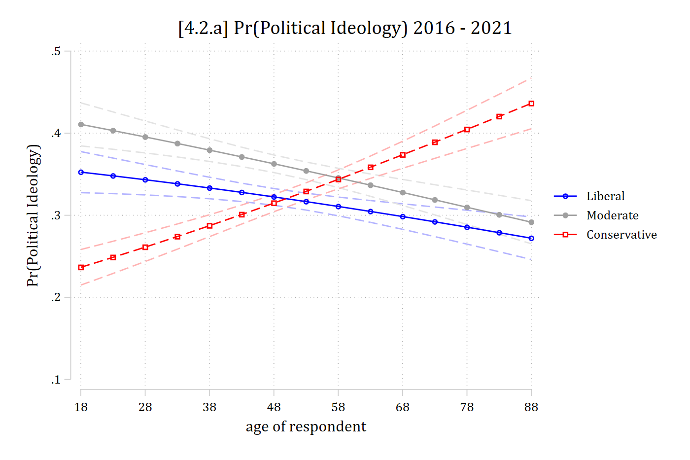
[4.2.a] Predicted probabilities of each political ideology by age with confidence intervals: Pr(liberal) falls from about 0.35 to 0.27, Pr(moderate) falls from about 0.41 to 0.29, and Pr(conservative) rises from about 0.24 to 0.44; the conservative line crosses the others in the late 40s to 50s.

It is now necessary to examine Pr(y = 1), Pr(y = 2), and Pr(y = 3) (the code for this graph is in 4.2)

Average marginal effects in multinomial logit

qui mlogit polviews3 c.age i.woman i.race3 i.college ///
    i.married i.parent c.faminc i.employed
est store pol3mod
mecompare age, amount(sd) model(pol3mod)
Predicting: Pr(polviews3)
Marginal effects (N_pol3mod=7823)

                                 |  ME #   Estimate         SE      P>|z|
---------------------------------+---------------------------------------
age + SD (centered)              |                                       
               Liberal - pol3mod |     1     -0.020      0.006      0.001
              Moderate - pol3mod |     2     -0.029      0.006      0.000
          Conservative - pol3mod |     3      0.049      0.006      0.000
pol3mod <- multinom(polviews3 ~ age + woman + race3 + college + married + parent +
  faminc + employed, data = gss, trace = FALSE)

avg_comparisons(pol3mod, variables = list(age = sd(gss$age)))

        Group Estimate Std. Error     z Pr(>|z|)    S   2.5 %  97.5 %
 Liberal       -0.0196    0.00596 -3.29  0.00102  9.9 -0.0313 -0.0079
 Moderate      -0.0294    0.00618 -4.75  < 0.001 18.9 -0.0415 -0.0173
 Conservative   0.0489    0.00606  8.08  < 0.001 50.4  0.0371  0.0608

Term: age
Type: probs
Comparison: +17.3603297947298
  • Because there are three outcome categories, there are three predicted probability curves for age (see plot above) and three AMEs for age (see above)
    • Do these AMEs correspond to your intuition from the graph?
  • But before we get to interpretation, some background
Back to top