5. Make groups easy to tell apart

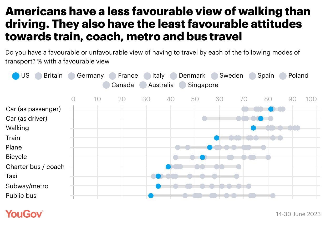
Bad graph example: cannot distinguish between symbols

YouGov dot plot of attitudes toward types of transport in eleven countries: the countries are marked with nearly identical gray dots, so they cannot be told apart.

use "https://tdmize.github.io/data/data/gss.dta", clear
(gss.dta | GSS 1972 - 2016 Data | DMV Workshop)
// 5.a - Overlay multiple densities for different groups
twoway kdensity wages if degree==0 || ///
       kdensity wages if degree==1 || ///
       kdensity wages if degree==2 || ///
       kdensity wages if degree==3 || ///
       kdensity wages if degree==4 ||, ///
       legend(order(1 "< High School" 2 "HS Degree" 3 "Junior College" ///
              4 "College Degree" 5 "Grad Degree")) ///
       ytitle("Density") xtitle("Hourly Wages") xlab(0(10)70) ///
       title("[5.a] Kernel-Density Plots of Hourly Wages Based on Educational 
Attainment") ///
       subtitle("Densities are group specific")

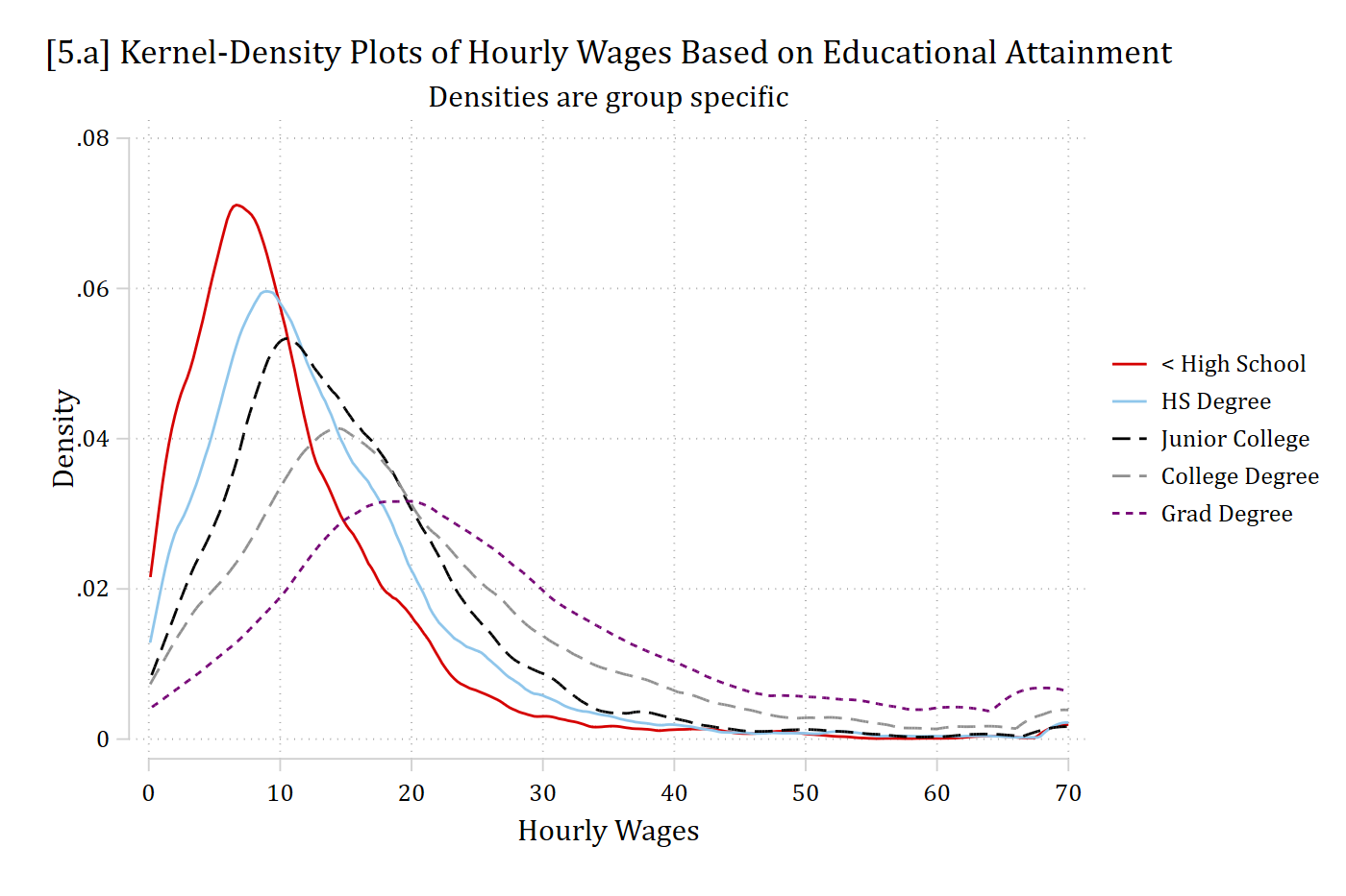
[5.a] Kernel density plots of hourly wages for five levels of education, each with its own color and line pattern: the less than high school curve peaks highest and earliest (near 7 dollars), and each higher degree peaks lower and farther to the right, with the graduate degree curve flattest and peaking near 20 dollars.

library(foreign)            # load Stata datasets
library(ggplot2)            # main graphics package
library(dplyr)              # data manipulation tools
library(cleanplots)         # Mize's graphics scheme

## Use cleanplots colors, markers, lines, and theme for all graphs ##
cleanplots_defaults()
theme_update(plot.title.position = "plot")   # titles start at left edge of graph

# General Social Survey Data
gss <- droplevels(read.dta("https://tdmize.github.io/data/data/gss.dta"))

# 5.a - Overlay multiple densities for different groups
# Use both colors and line patterns so the five groups are easy to tell apart
degree_labels <- c("< High School", "HS Degree", "Junior College",
                   "College Degree", "Grad Degree")

ggplot(filter(gss, !is.na(degree)), aes(x = wages, color = degree, linetype = degree)) +
  geom_density(key_glyph = "path") +
  labs(x = "Hourly Wages", y = "Density", color = "", linetype = "",
       title = "[5.a] Kernel-Density Plots of Hourly Wages Based on Educational Attainment",
       subtitle = "Densities are group specific") +
  scale_color_cleanplots(labels = degree_labels) +
  scale_linetype_cleanplots(labels = degree_labels) +
  scale_x_continuous(breaks = seq(0, 70, 10))
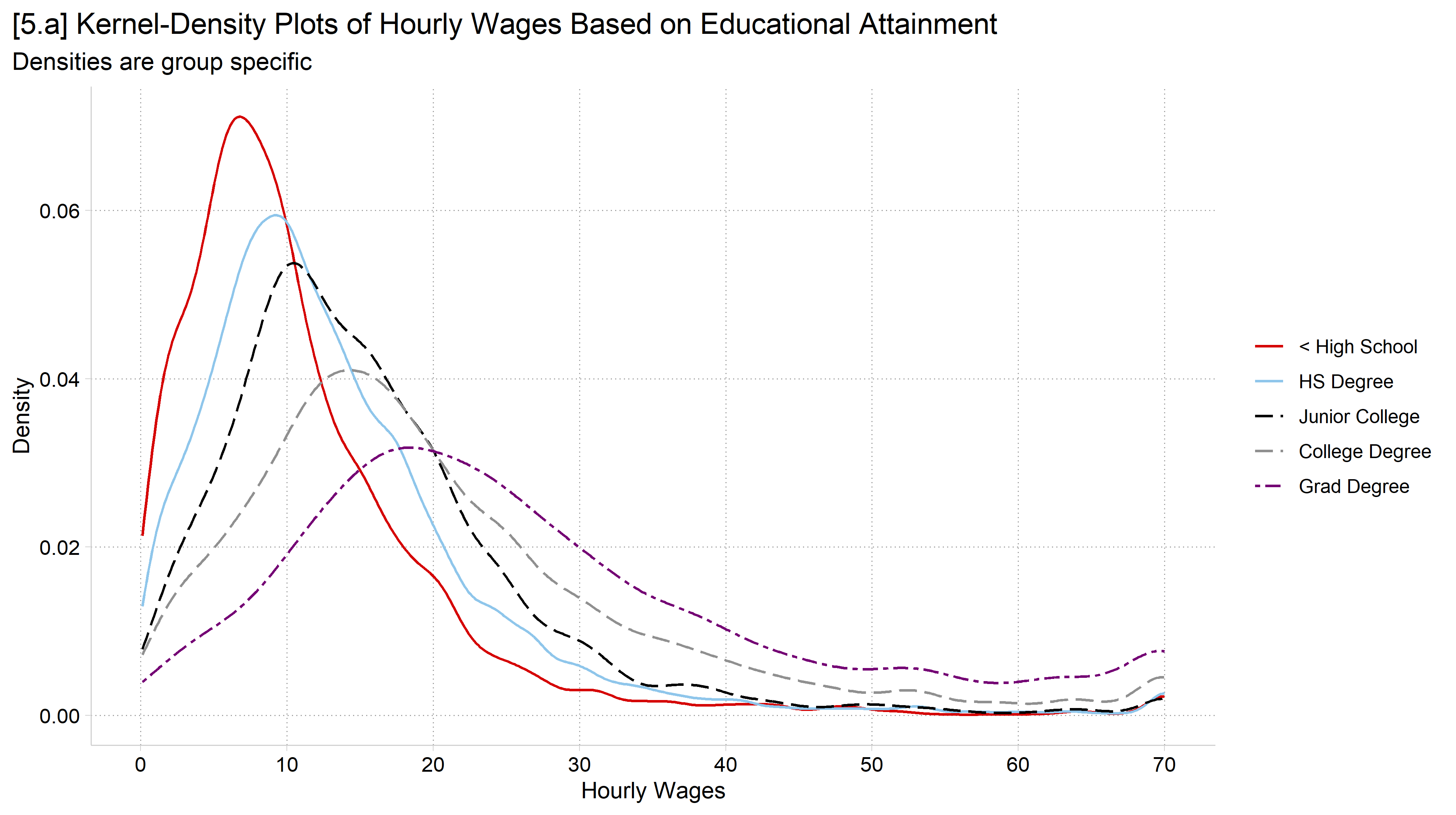
[5.a] Kernel density plots of hourly wages for five levels of education, each with its own color and line pattern: the less than high school curve peaks highest and earliest, and each higher degree peaks lower and farther to the right, with the graduate degree curve flattest.

use "https://tdmize.github.io/data/data/hrs_si.dta", clear
(Health and Retirement Study 1992-2022 - Cleaned for MCAP SI)
egen byte in1992 = max(year == 1992), by(hhidpn)
* Value labels for year so coefplot labels each wave with its year
levelsof year, local(yrs)
1992 1994 1996 1998 2000 2002 2004 2006 2008 2010 2012 2014 2016 2018 2020 2022
foreach y of local yrs {
    label define yearlab `y' "`y'", add
}
label values year yearlab
// 5.b - Mean cognitive test score by year, separately for men and women
*coefplot offsets the groups so their confidence intervals do not overlap
qui regress cog ibn.year if in1992 & woman == 0, nocons
est store cog_men
qui regress cog ibn.year if in1992 & woman == 1, nocons
est store cog_wom
coefplot (cog_men, label("Men")) (cog_wom, label("Women")), ///
    vertical ylabel(12(1)18) ///
    xtitle("Year") ytitle("Cognitive test score") ///
    title("[5.b] Performance on a cognitive test over time, by gender") ///
    subtitle("Means and 95% confidence intervals")

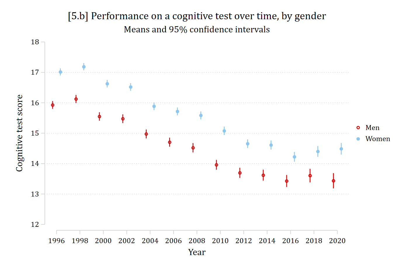
[5.b] Mean cognitive test scores with 95% confidence intervals for men (red) and women (light blue) in each HRS wave from 1996 to 2020: scores decline over time for both, from about 16 to 13.5 for men and from about 17 to 14.5 for women, with women higher in every wave.

# Health and Retirement Study Data
hrs <- read.dta("https://tdmize.github.io/data/data/hrs_si.dta")

# Quick work to flag only those included in first HRS wave
ids_1992 <- hrs %>%
  filter(year == 1992) %>%
  pull(hhidpn) %>% unique()

hrs_filtered <- hrs %>%
  filter(hhidpn %in% ids_1992)

# 5.b - Mean cognitive test score by year, separately for men and women
# position_dodge( ) offsets the groups so their confidence intervals do not overlap
dodge <- position_dodge(width = .5)

ggplot(filter(hrs_filtered, !is.na(cog)),
       aes(x = factor(year), y = cog, color = woman, group = woman)) +
  stat_summary(fun = mean, geom = "point", size = 2.5, position = dodge) +
  stat_summary(fun.data = mean_cl_normal, geom = "errorbar", width = .2, position = dodge) +
  labs(x = "Year", y = "Cognitive test score", color = "",
       title = "[5.b] Performance on a cognitive test over time, by gender",
       subtitle = "Means and 95% confidence intervals") +
  scale_y_continuous(breaks = seq(12, 18, 1)) + coord_cartesian(ylim = c(12, 18))

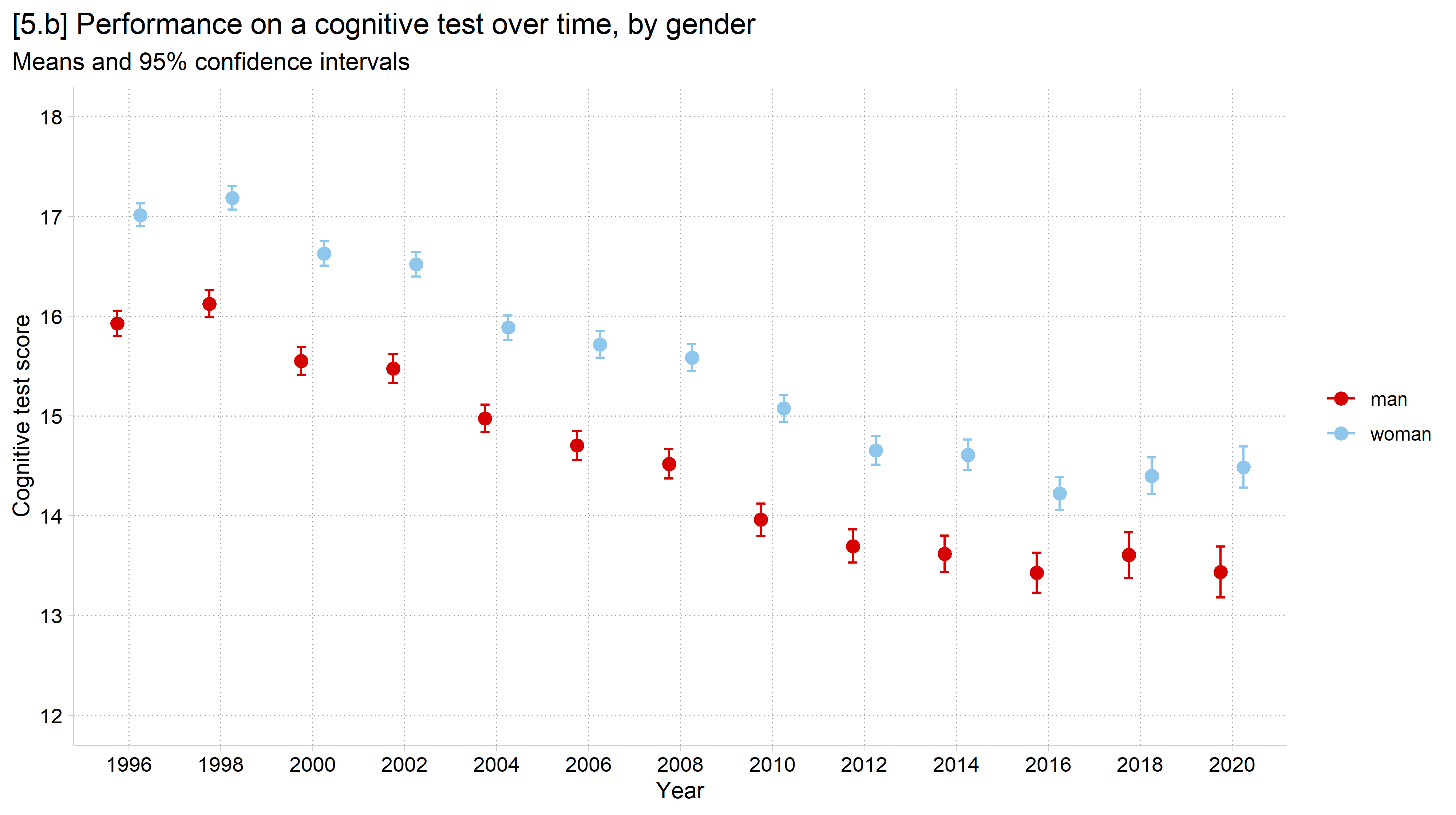
[5.b] Mean cognitive test scores with 95% confidence intervals for men and women in each HRS wave from 1996 to 2020: scores decline over time for both, with women higher in every wave.

General advice: color

The color scheme (sequence of colors) on your graph should work for you—not against you

  • Nominal (unordered) color schemes are best when you want distinct visual separation for each aspect of the plot
    • E.g., For a nominal variable such as race/ethnicity or religion
  • Ordinal (sequential) color schemes work best for representing data that has a natural order
    • E.g., Age groups (e.g., generations) or Likert response options
  • Diverging color schemes have a natural midpoint and diverge to both extremes
    • E.g., Political views

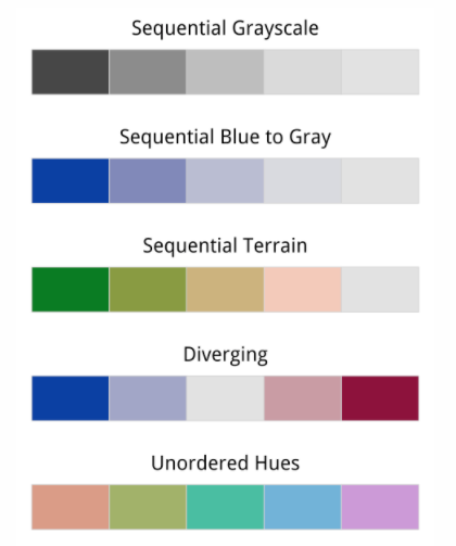
Example color schemes: sequential grayscale, sequential blue to gray, sequential terrain, diverging, and unordered hues.

*Color chart from Healy 2018

  • Color alone can usually be used to distinguish between approximately 4–5 different lines/markers (see the color limits section below)
    • Once you have 5+, you should also distinguish between lines/markers with different patterns (e.g., solid/dashed) and/or symbols (e.g., o, △, ☐)
  • The main colors on a graphic should be distinguishable even when printed in black & white
    • Most journals allow color figures for the online version
      • However, most only print in black & white
    • But if your color scheme also works in black & white, no need to make two figures (more in the Graphics Themes section)
  • Avoid combining red and green
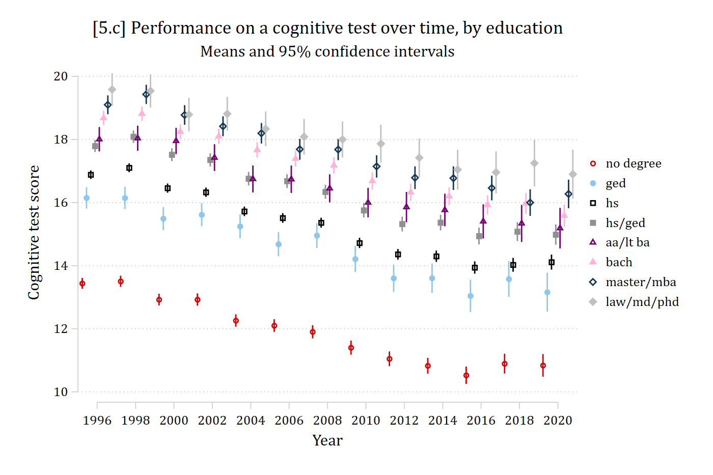
// 5.c - Many groups: cleanplots changes marker shapes in addition to color
local plots
forvalues d = 0/7 {
    qui regress cog ibn.year if in1992 & degree == `d', nocons
    est store cog_deg`d'
    local lab : label (degree) `d'
    local plots `plots' (cog_deg`d', label("`lab'"))
}
coefplot `plots', vertical ylabel(10(2)20) ///
    xtitle("Year") ytitle("Cognitive test score") ///
    title("[5.c] Performance on a cognitive test over time, by education") ///
    subtitle("Means and 95% confidence intervals")

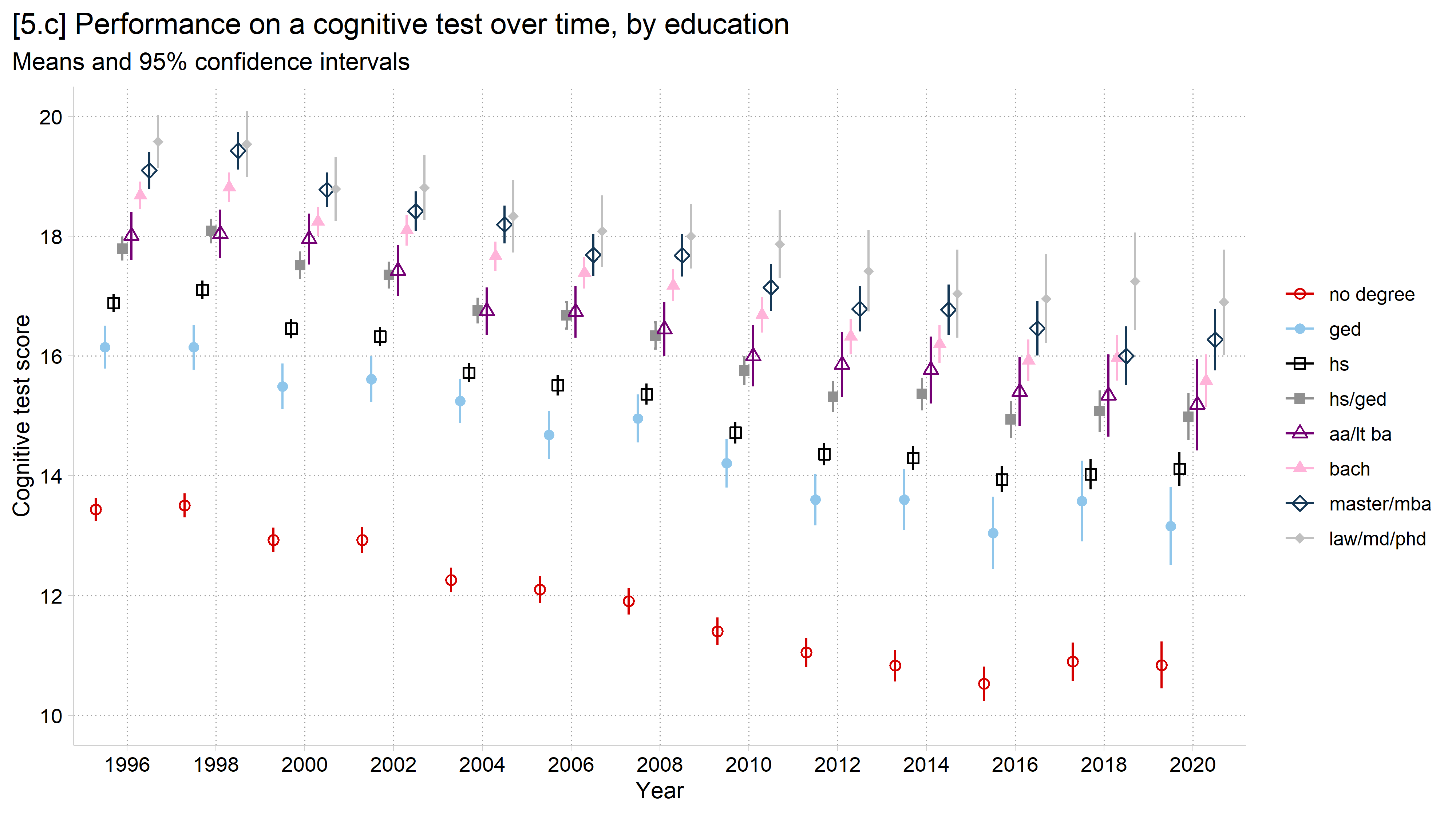
[5.c] Mean cognitive test scores with 95% confidence intervals for eight education groups in each wave from 1996 to 2020, each group with its own color and marker shape: scores decline over time in every group, and groups with more education score higher: the no degree group falls from about 13.5 to about 11, while the law/md/phd group stays highest, between about 17 and 19.5.

# 5.c - Many groups: need to change marker shapes in addition to color
dodge <- position_dodge(width = .8)

ggplot(filter(hrs_filtered, !is.na(cog), !is.na(degree)),
       aes(x = factor(year), y = cog, color = degree, shape = degree, group = degree)) +
  stat_summary(fun = mean, geom = "point", size = 2, position = dodge) +
  stat_summary(fun.data = mean_cl_normal, geom = "errorbar",
               width = 0.2, position = dodge) +
  labs(x = "Year",
       y = "Cognitive test score",
       color = "", shape = "",
       title = "[5.c] Performance on a cognitive test over time, by education",
       subtitle = "Means and 95% confidence intervals") +
  scale_shape_cleanplots() +
  scale_y_continuous(breaks = seq(10, 20, 2)) + coord_cartesian(ylim = c(10, 20))

[5.c] Mean cognitive test scores with 95% confidence intervals for eight education groups in each wave from 1996 to 2020, each group with its own color and marker shape: scores decline over time in every group, and groups with more education score higher.

Nominal scheme color limits

  • With a nominal scheme, it is hard to distinguish more than about 6 colors and “…the task of matching colors to categories becomes too burdensome to be useful…” (Wilke 2019 p.234)
use "https://tdmize.github.io/data/data/cgr.dta", clear
(CGR Prolific | Intersectionality Stereotype Content | 2024-04-17 : TDM)
*collapse to means by experimental condition
collapse compSS warmSS if ordcond == 2, by(cond)
list
     +--------------------------------------------+
     |                 cond     compSS     warmSS |
     |--------------------------------------------|
  1. |            White Men   6.549223    5.25285 |
  2. |          White Women   5.473596   5.839888 |
  3. |            Black Men   5.117368   4.119473 |
  4. |          Black Women   5.459799   4.954774 |
  5. |           Latino Men   5.390164   4.720219 |
     |--------------------------------------------|
  6. |         Latina Women   5.254082   5.345408 |
  7. |            Asian Men    6.30904   4.957627 |
  8. |          Asian Women   5.614286    5.46798 |
  9. |          Chinese Men   6.247938   4.464949 |
 10. |        Chinese Women   5.765608   5.016931 |
     |--------------------------------------------|
 11. |         Japanese Men   6.323333   5.127222 |
 12. |       Japanese Women   5.297369   5.784211 |
 13. |           Korean Men   6.034391   4.838624 |
 14. |         Korean Women   5.377835   5.225258 |
 15. |           Indian Men   5.909645   4.438071 |
     |--------------------------------------------|
 16. |         Indian Women   5.112088   5.265385 |
 17. |        Pakistani Men   5.328272   3.594764 |
 18. |      Pakistani Women   3.648925   4.256989 |
 19. |   Middle Eastern Men   5.608287    3.41768 |
 20. | Middle Eastern Women   3.773846   4.290769 |
     |--------------------------------------------|
 21. |          Iranian Men    5.65873   3.669841 |
 22. |        Iranian Women   3.827778   4.027778 |
 23. |    Saudi Arabian Men   5.830457   3.422843 |
 24. |  Saudi Arabian Women    3.29901   4.045545 |
 25. |          Mexican Men       5.35    4.62043 |
     |--------------------------------------------|
 26. |        Mexican Women   4.929744   5.235384 |
     +--------------------------------------------+
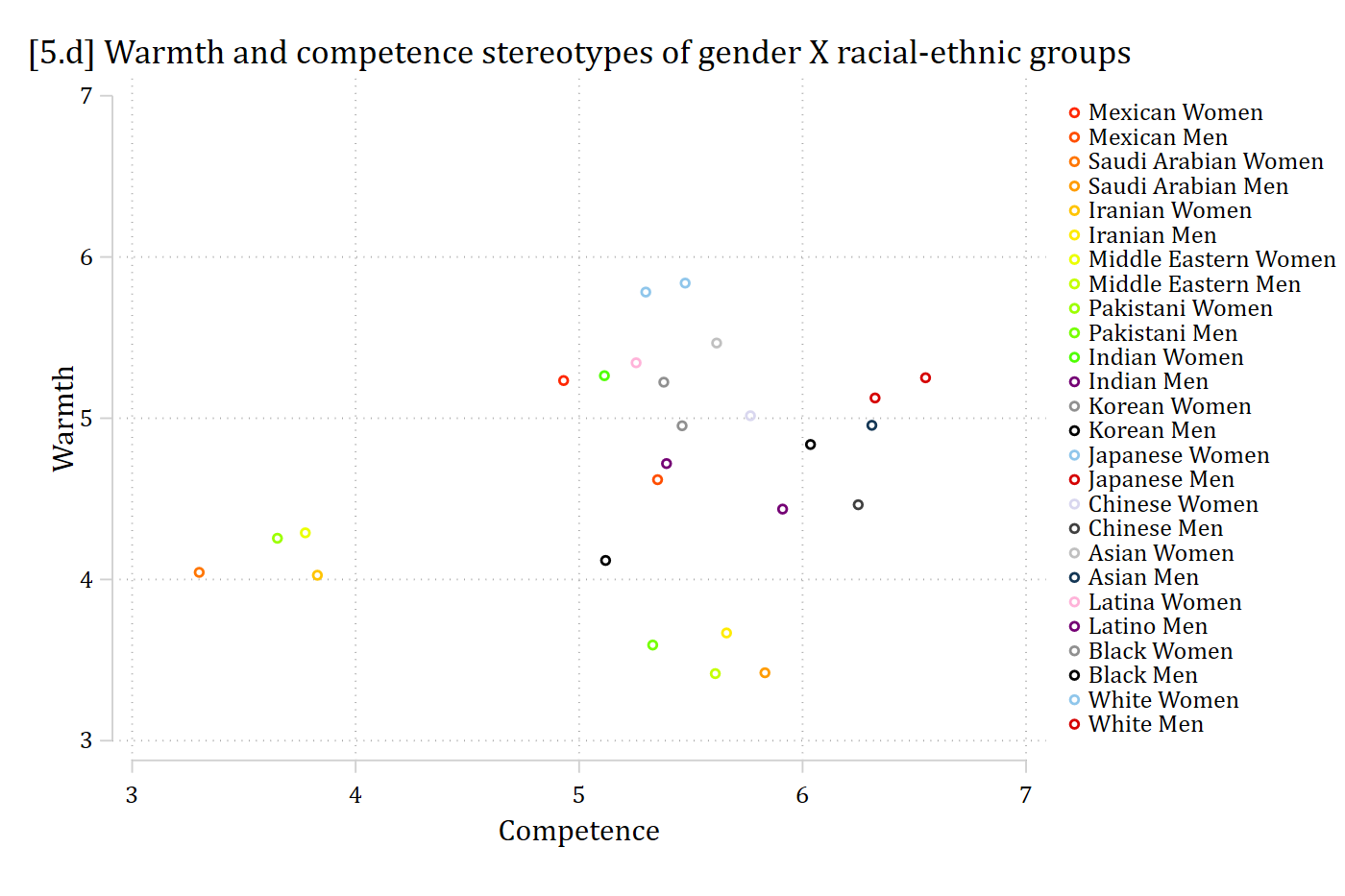
// 5.d - discrete color for each marker (too many colors to understand)
twoway scatter warmSS compSS, ///
        colorvar(cond) colordiscrete coloruseplegend ///
        zlabel(, valuelabel) colorrule(phue) ///
    ytitle("Warmth") xtitle("Competence") ylab(3(1)7) xlab(3(1)7) ///
    title("[5.d] Warmth and competence stereotypes of gender X racial-ethnic g
roups")

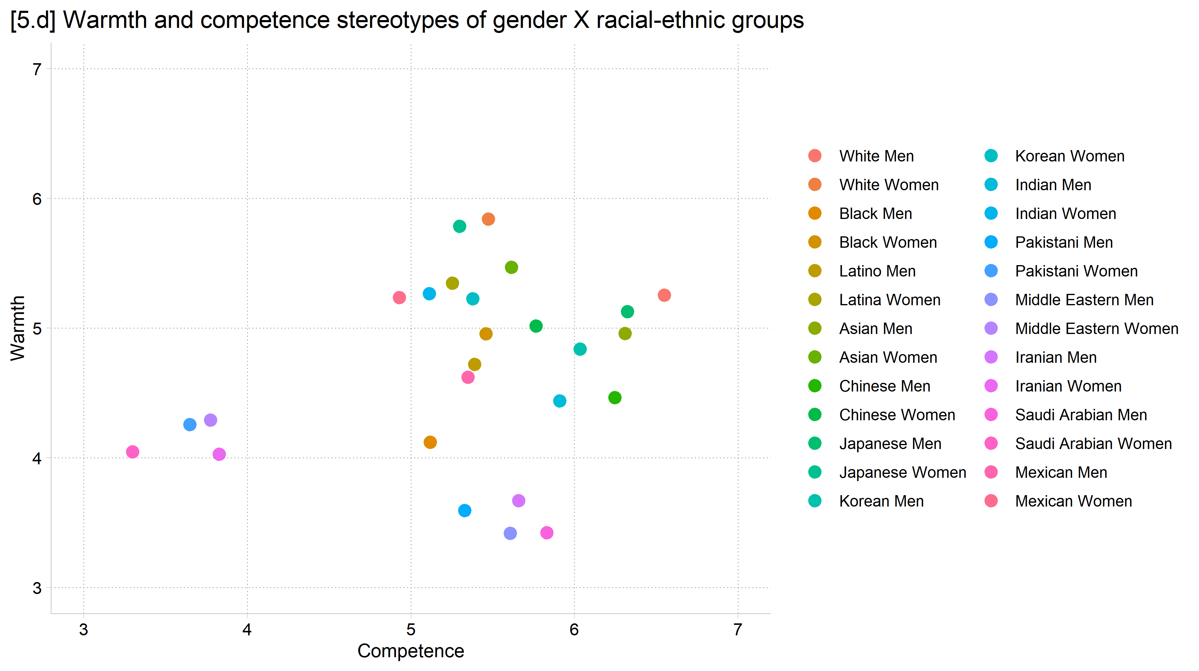
[5.d] Scatterplot of mean warmth by mean competence stereotypes for 26 gender by racial-ethnic groups, each group a different color with a 26-entry legend: the colors are too similar to match the points to the groups.

# Mize 2025 SPQ stereotypes data
cgr <- read.dta("https://tdmize.github.io/data/data/cgr.dta")

# 5.d & 5.e - Calculate experimental condition means
means_by_condition <- cgr %>%
  filter(ordcond == "Second Order") %>%
  droplevels() %>%
  group_by(cond) %>%
  summarise(mean_warmth     = mean(warmSS, na.rm = TRUE),
            mean_competence = mean(compSS, na.rm = TRUE))
means_by_condition
# A tibble: 26 × 3
   cond          mean_warmth mean_competence
   <fct>               <dbl>           <dbl>
 1 White Men            5.25            6.55
 2 White Women          5.84            5.47
 3 Black Men            4.12            5.12
 4 Black Women          4.95            5.46
 5 Latino Men           4.72            5.39
 6 Latina Women         5.35            5.25
 7 Asian Men            4.96            6.31
 8 Asian Women          5.47            5.61
 9 Chinese Men          4.46            6.25
10 Chinese Women        5.02            5.77
# ℹ 16 more rows
# 5.d - Too many colors to understand (not recommended)
ggplot(means_by_condition, aes(x = mean_competence, y = mean_warmth, color = cond)) +
  geom_point(size = 3) +
  scale_color_hue() +    # a distinct color for each of the 26 groups
  labs(x = "Competence", y = "Warmth", color = "",
       title = "[5.d] Warmth and competence stereotypes of gender X racial-ethnic groups") +
  scale_x_continuous(breaks = seq(3, 7, 1), limits = c(3, 7)) +
  scale_y_continuous(breaks = seq(3, 7, 1), limits = c(3, 7))

[5.d] Scatterplot of mean warmth by mean competence stereotypes for 26 gender by racial-ethnic groups, each group a different color with a 26-entry legend: the colors are too similar to match the points to the groups.

Data from Mize 2025

  • With many categories, can be more effective to directly label the markers/lines
// 5.e - With so many groups, better to just directly label points
twoway scatter warmSS compSS, mlabel(cond) ///
    ytitle("Warmth") xtitle("Competence") ylab(3(1)7) xlab(3(1)7) ///
    title("[5.e] Warmth and competence stereotypes of gender X racial-ethnic g
roups")

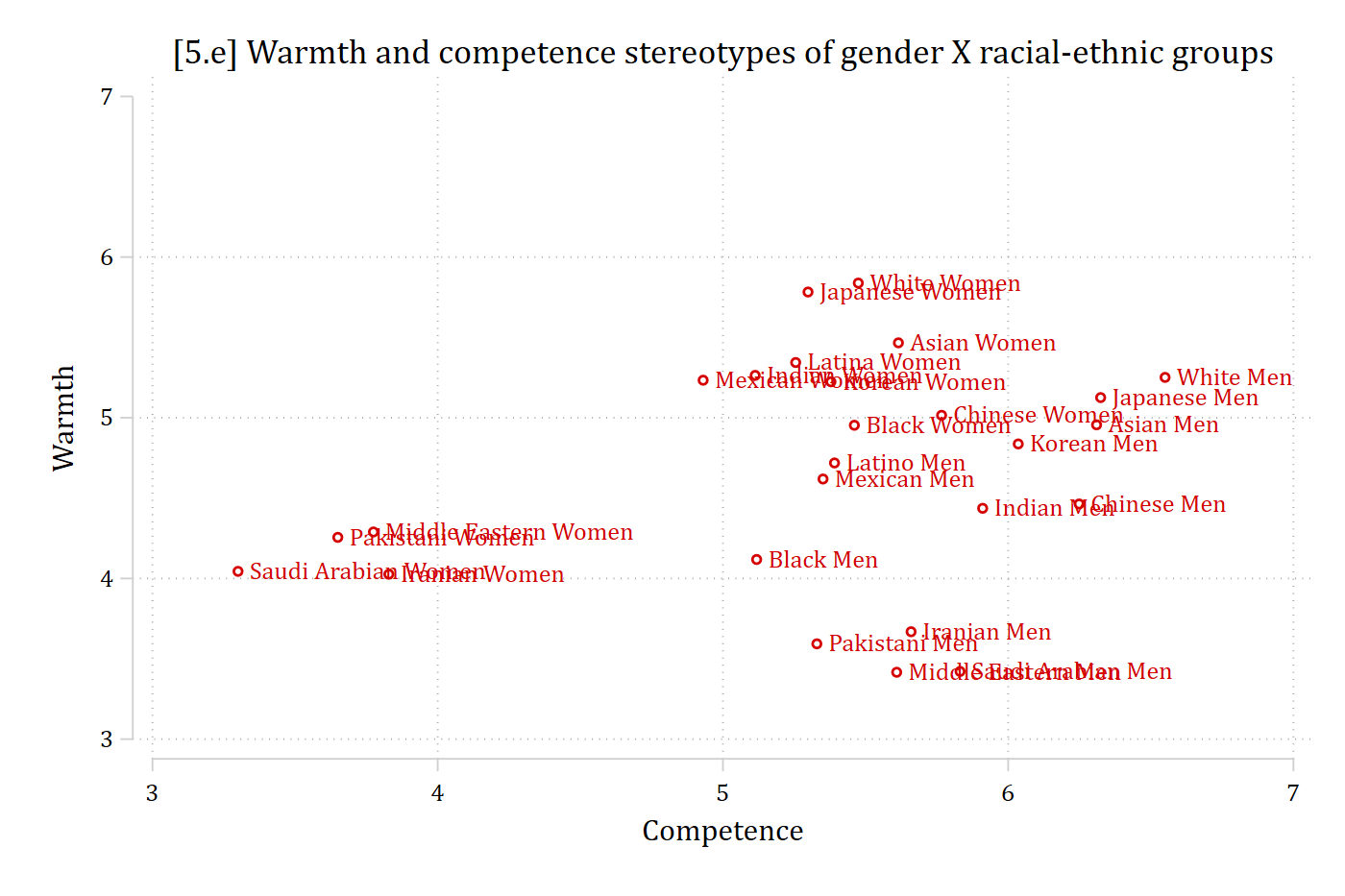
[5.e] The same scatterplot with each point labeled directly with its group name: White Men and Asian Men are rated most competent, Pakistani, Iranian, Saudi Arabian, and Middle Eastern Women least competent, and the Middle Eastern, Saudi Arabian, Pakistani, and Iranian Men least warm.

# 5.e - With so many groups, better to just directly label points
ggplot(means_by_condition, aes(x = mean_competence, y = mean_warmth, label = cond)) +
  geom_point(size = 3) +
  geom_text(vjust = -0.8, size = 3.5) +
  labs(x = "Competence", y = "Warmth",
       title = "[5.e] Warmth and competence stereotypes of gender X racial-ethnic groups") +
  scale_x_continuous(breaks = seq(3, 7, 1), limits = c(3, 7)) +
  scale_y_continuous(breaks = seq(3, 7, 1), limits = c(3, 7))

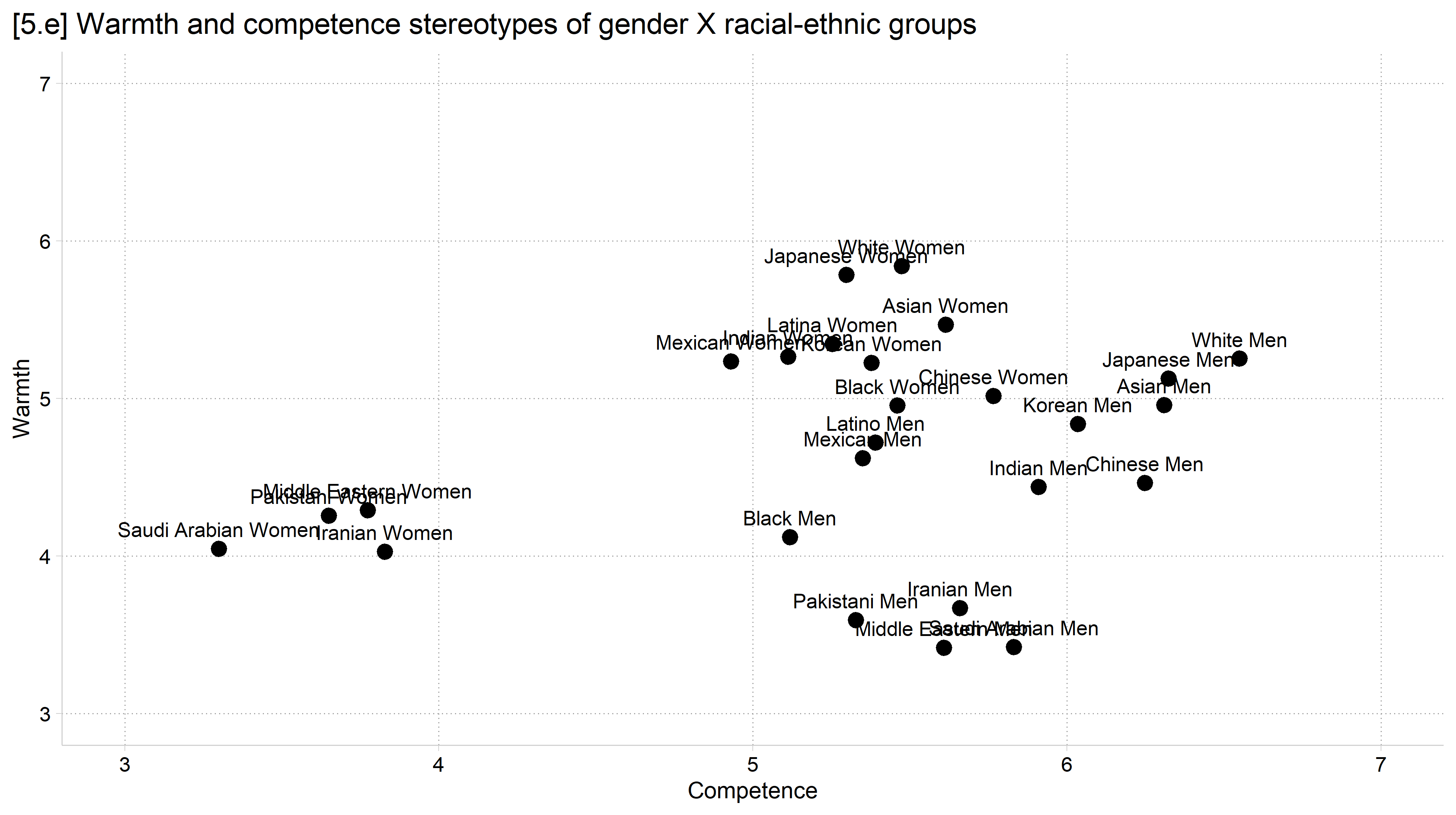
[5.e] The same scatterplot with each point labeled directly with its group name: White Men and Asian Men are rated most competent, Pakistani, Iranian, Saudi Arabian, and Middle Eastern Women least competent, and the Middle Eastern, Saudi Arabian, Pakistani, and Iranian Men least warm.

Data from Mize 2025

Creating figures considerate of colorblindness

  • About 5% of the population has some form of colorblindness (red/green being the most common which is why you should always avoid having red and green together on your figure… looking at you stcolor)
    • This excellent website Coloring for Colorblindness lets you check your color schemes to see how they will be viewed for those who are colorblind
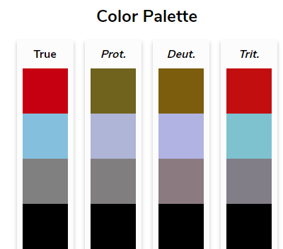
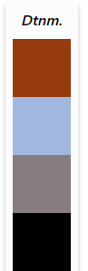
      • Below is an example for how the first four default cleanplots colors look to individuals with various types of colorblindness

The first four cleanplots colors (red, light blue, gray, black) as seen with typical vision and with protanopia, deuteranopia, and tritanopia: the four colors stay distinct in every column. The same four colors as seen with deuteranomaly.

Nominal and ordinal color palettes

  • Most graphics themes’ palettes are nominal
    • I.e., They do not imply ordering by the color choices
    • okabe_ito and cleanplots are nominal palettes
  • It is sometimes useful to use an ordinal palette to have the visual reflect the ordering in the variable (e.g., for educational degrees)
    • The viridis and cividis palettes are my preferred ordinal palettes
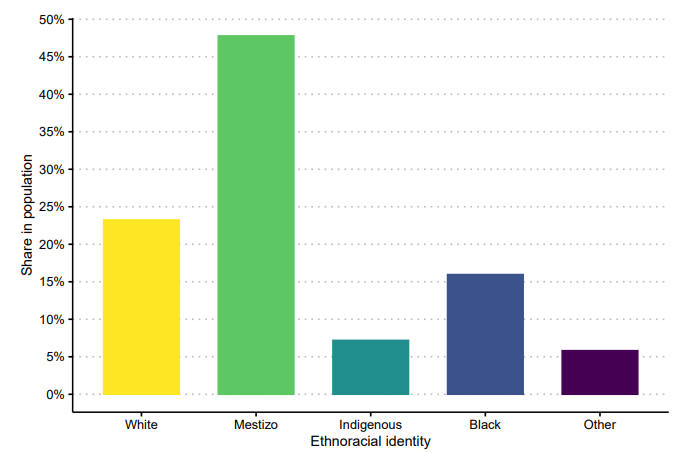
    • Note you should not use an ordinal palette for a nominal variable (falsely implies ordering)

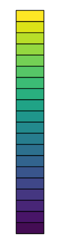
The viridis ordinal palette, running from yellow through green and teal to dark purple.

Bar chart of a nominal race-ethnicity variable drawn in an ordinal palette, crossed out with a red X.

Should use a nominal palette for a race-ethnicity variable

use "https://tdmize.github.io/data/data/hrs_si.dta", clear
(Health and Retirement Study 1992-2022 - Cleaned for MCAP SI)
// 5.f - Ordinal (viridis) colors for an ordered variable: cleanplots8v scheme
graph bar (mean) dzcount, over(degree) asyvars showyvars legend(off) ///
    yvaroptions(label(angle(45))) ///
    ytitle("Count of chronic diseases") ///
    title("[5.f] Average chronic disease count by educational attainment") ///
    subtitle("Colors are from cleanplots ordinal viridis scheme") ///
    scheme(cleanplots8v)

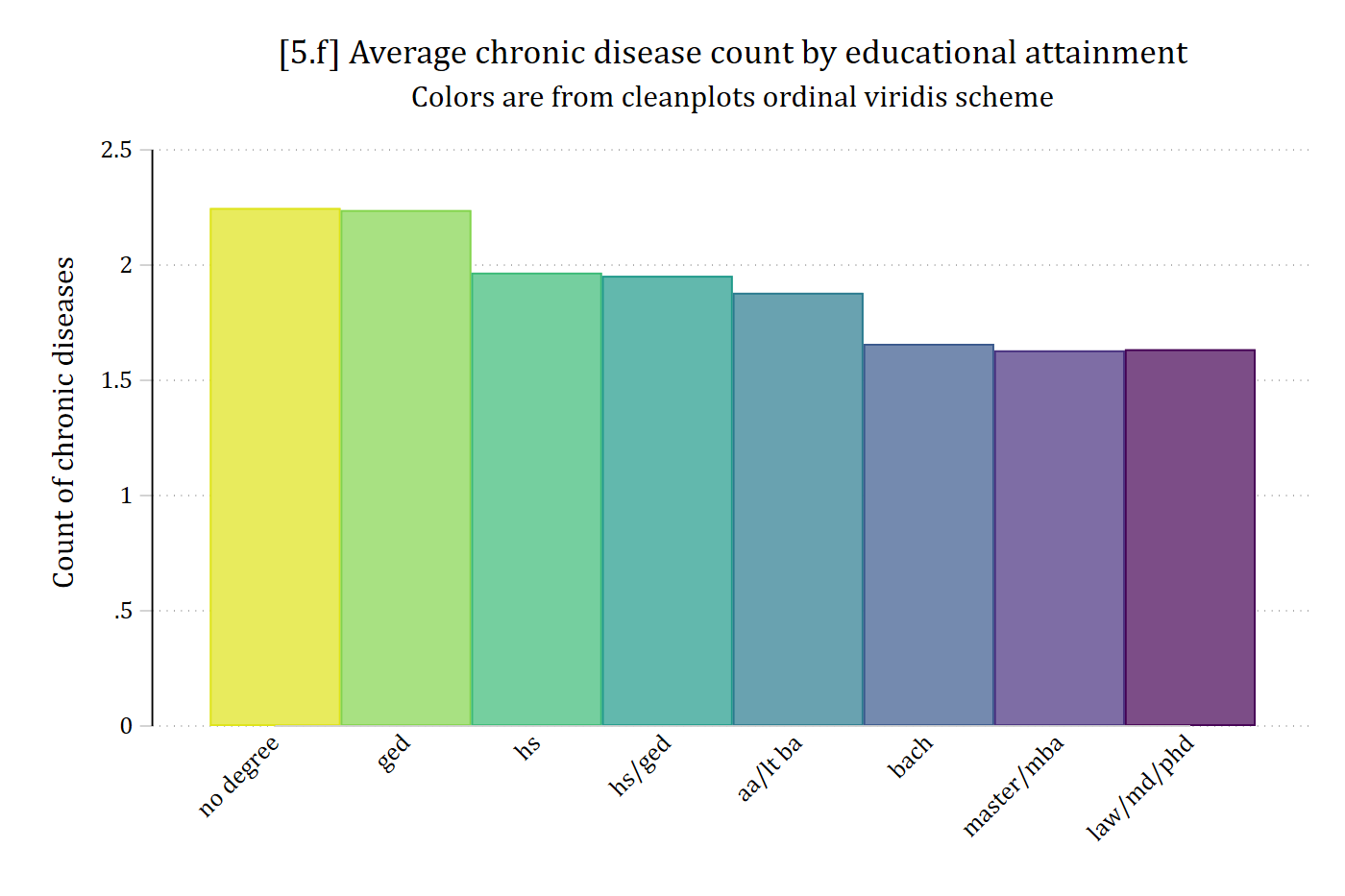
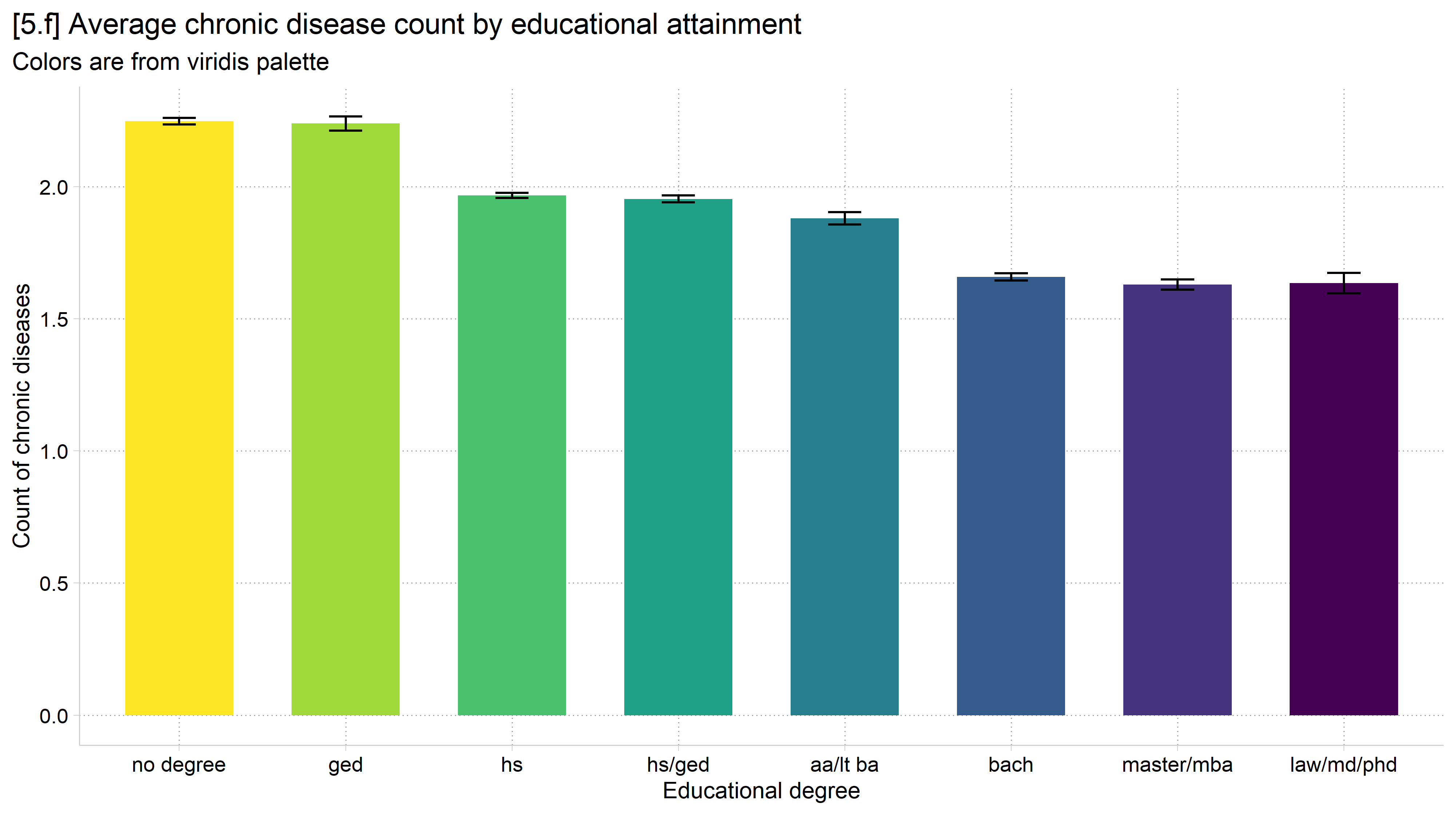
[5.f] Bar chart of the average count of chronic diseases for eight education groups in ordinal viridis colors, from light yellow for no degree to dark purple for law/md/phd: the average falls from about 2.25 with no degree to about 1.6 for the highest degrees.

# 5.f - Ordinal (viridis) palette for an ordered variable
ggplot(filter(hrs, !is.na(dzcount), !is.na(degree)),
       aes(x = degree, y = dzcount, fill = degree)) +
  stat_summary(fun = mean, geom = "bar", width = 0.65) +
  stat_summary(fun.data = mean_cl_normal, geom = "errorbar", width = 0.2) +
  labs(x = "Educational degree",
       y = "Count of chronic diseases",
       title = "[5.f] Average chronic disease count by educational attainment",
       subtitle = "Colors are from viridis palette") +
  theme(legend.position = "none") +
  scale_fill_viridis_d(direction = -1)

[5.f] Bar chart of the average count of chronic diseases for eight education groups in ordinal viridis colors, from light yellow for no degree to dark purple for law/md/phd, with 95% confidence intervals: the average falls as education rises.

*Note ordering of colors. Logic = darker, more saturated colors = more of construct

Back to top