Appendix 2B: Logged DV Regression Models
2.9 Logged DV regression models
- A linear regression model can be used in which the dependent variable has been logged and then a linear regression model has been fit
- E.g., Often used when income or wages is the DV due to a strong positive skew
- Logged DV models introduce complications for interpretation for:
- Coefficients
- Predictions
- Marginal effects
- Many of these complications mirror those in binary regression models (e.g., logit and probit)
- Linear regression models with logged DVs are inherently nonlinear via a transformation of the dependent variable
- The DV is the natural log of the original variable; e.g. ln(wages) is a common DV in labor market analyses
- Need a refresher on logs and natural logs? The Wikipedia article is quite good. The natural logarithm has the mathematical constant e (≈2.718) as its base
\[\log_{e}x = \ln(x) \qquad c = \ln(x) \qquad e^{c} = x \qquad \ln(e) = 1 \qquad e^{1} = e\]
- Why log your DV? Positively skewed DVs are a common motivation*
- Recall that regression models expectations (means) and conditional expectations. Is the mean a good summary of a positively skewed distribution? (See graph below)
*Poisson models are a possible alternative (Gould 2011). More on these in the Count section of the class
usetdm smi_gss, clearLoading dataset...
(SMI | Mize 2016 ASR | GSS Data on Sexual Behavior and Wages)sum wages logwages Variable | Obs Mean Std. dev. Min Max
-------------+---------------------------------------------------------
wages | 13,064 18.81297 38.21546 1 1773.6
logwages | 13,064 2.541626 .8696813 0 7.480767hist wages if wages <= 150, percent title("[2.8.a] Distribution of Wages") ///
fc(none) xline(18.81, lcolor(red) lstyle(solid) lwidth(thick)) ///
normal text(10 40 "mean = $18.81")(bin=41, start=1, width=3.5150627)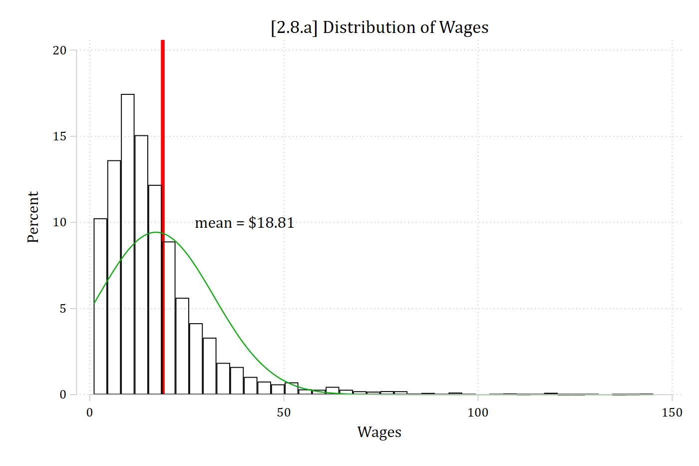
Is the mean a good summary of this distribution?
hist logwages, percent title("[2.8.b] Distribution of Logged Wages") ///
    fc(none) xline(2.54, lcolor(red) lstyle(solid) lwidth(thick)) ///
    normal text(9 4 "mean = 2.54")
(bin=41, start=0, width=.18245773)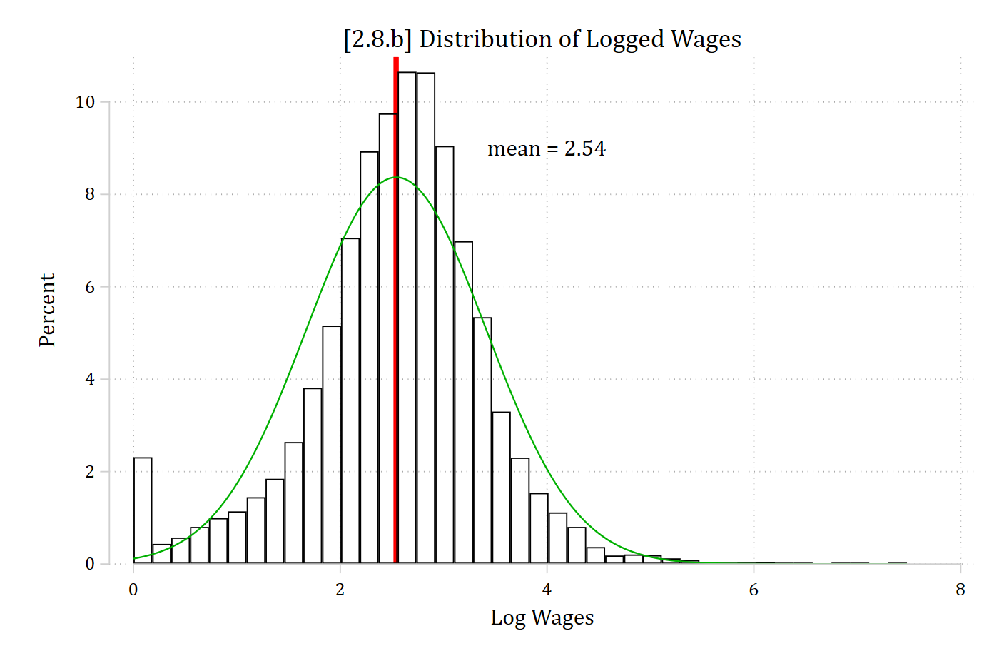
Logging positively skewed variables helps normalize the distribution/pull in outliers
Logged DV regression models
- First, a little bit more math review:
\[\exp(a + b) = \exp(a)*\exp(b)\]
\[\log\left\lbrack \exp(a + b) \right\rbrack = a + b\]
- An exponential model is multiplicative on the y metric
\[y = \exp\left( \beta_{0} + \beta_{k}x_{k} + \beta_{2}x_{2} + \varepsilon \right)\]
\[= \exp(\beta_{0})\exp(\beta_{k}x_{k})\exp(\beta_{2}x_{2})\exp(\varepsilon)\]
- To get back to a model that looks like linear regression, we can take the log of the entire model making the model loglinear [y becomes ln(y)]
- The model becomes additive—but only in the ln(y) metric
Interpreting logged DV regression models
- The model after taking the natural log:
\[\ln(y) = \ln\left\lbrack \exp\left( \beta_{0} + \beta_{k}x_{k} + \beta_{2}x_{2} + \varepsilon \right) \right\rbrack\]
\[= \beta_{0} + \beta_{k}x_{k} + \beta_{2}x_{2} + \varepsilon\]
- \(\beta_{k}\) is interpreted as:
- For a unit increase in xk, the log of y is expected to increase by βk units, holding other variables constant
- This is an additive effect (i.e. each one unit increase in xk leads to an additional βk units)
- However, a change in the log of y is often substantively unclear
- E.g. Do you want to interpret effects in terms of the log of wages?
- We can instead interpret factor changes: multiplicative effects in the y metric (defined below)
Factor change in y interpretations
- Start value: Let y(xk, \(\mathbf{x}_{- k}\)) be the value of y focusing on xk:
\[y\left( x_{k},\mathbf{x}_{- k} \right) = \exp(\beta_{0} + \beta_{k}x_{k} + \beta_{2}x_{2} + \varepsilon)\]
\[= \exp(\beta_{0})\exp(\beta_{k}x_{k})\exp(\beta_{2}x_{2})\exp(\varepsilon)\]
- End value: y(xk+1, \(\mathbf{x}_{- k}\)) is the value of y after increasing xk by 1:
\[y\left( x_{k} + 1,\mathbf{x}_{- k} \right) = \exp(\beta_{0})\exp\left\lbrack \beta_{k}\left( x_{k} + 1 \right) \right\rbrack\exp(\beta_{2}x_{2})\exp(\varepsilon)\]
\[= \exp(\beta_{0})\exp(\beta_{k}x_{k})\exp(\beta_{k})\exp(\beta_{2}x_{2})\exp(\varepsilon)\]
- The ratio y(xk+1, \(\mathbf{x}_{- k}\))/y(xk, \(\mathbf{x}_{- k}\)) is the factor change in y for a unit increase in xk; it is a multiplicative effect with an increase in xk leading to y changing by a factor of \(\exp(\beta_{k})\):
\[\frac{y_{end}}{y_{start}} = \frac{y(x_{k} + 1,\ \mathbf{x}_{- k})}{y(x_{k},\ \mathbf{x}_{- k})}\]
\[= \frac{\exp\left( \beta_{0} \right)\exp\left( \beta_{k}x_{k} \right)\exp\left( \beta_{k} \right)\exp\left( \beta_{2}x_{2} \right)\exp(\varepsilon)}{\exp\left( \beta_{0} \right)\exp\left( \beta_{k}x_{k} \right)\exp\left( \beta_{2}x_{2} \right)\exp(\varepsilon)} = \exp(\beta_{k})\]
Interpreting logged DV regression models with factor changes
What is a “factor change?” Multiplicative effect:
Need to know the starting value. E.g. y = 10
- Factor change of 2: y is doubled or twice as large: 2*10 = 20
- Factor change of 0.5: y is reduced in half: 0.5*10 = 5
Factor change ranges
Factor changes larger than 1 indicate a positive effect; there is no upper ceiling on how large the factor change can be
Factor changes between 0 and 1 indicate a negative effect; there is a floor at 0
- If y is 2 times larger: y doubles (i.e. *2)
- If y is 1.5 times larger: y increases by one and a half times (i.e. *1.5)
- If y is 0.5 times smaller: y is reduced by half (i.e. *0.5)
- If y is 0 times smaller: y is reduced to 0 regardless of its start value (i.e. * 0)
Factor change interpretations
- Factor change interpretation: for a unit increase in xk, y is expected to be exp(βk) times larger (or smaller), holding other variables constant
- The factor change is in the y metric [not ln(y)] but is multiplicative; not additive
- For multiplicative effects: Take the starting value and multiply it by exp(βk) to determine the ending value
- For example, consider a model for the unconditional gender wage gap in 2018:
use "https://tdmize.github.io/data/data/cda_gss", clear(cda_gss.dta | GSS 1972-2021 CDA - Categorical Data Analysis | date created 202
> 3)gen logwages = ln(wages)(35,686 missing values generated)reg logwages i.woman if year == 2018 Source | SS df MS Number of obs = 1,176
-------------+---------------------------------- F(1, 1174) = 23.13
Model | 23.8153521 1 23.8153521 Prob > F = 0.0000
Residual | 1208.56142 1,174 1.02943903 R-squared = 0.0193
-------------+---------------------------------- Adj R-squared = 0.0185
Total | 1232.37677 1,175 1.0488313 Root MSE = 1.0146
------------------------------------------------------------------------------
logwages | Coefficient Std. err. t P>|t| [95% conf. interval]
-------------+----------------------------------------------------------------
woman |
Women | -0.285 0.059 -4.810 0.000 -0.401 -0.169
_cons | 2.646 0.042 62.312 0.000 2.562 2.729
------------------------------------------------------------------------------di exp(-0.285).75201425- The factor change (\(\exp\left( \beta_{woman} \right) = 0.75\)) can be interpreted as either*:
Women’s hourly wages are lower than men’s by a factor of 0.75
Women earn 0.75 times less than men
- Is 0.75 a big effect? Small effect? Medium-sized effect? Effects in a multiplicative metric make contextualizing effect sizes difficult
- The size of the effect depends on where you start!
- In this case, the starting value for xwoman is 0 which is men (i.e. they are the reference group)
- For example:
- If men’s hourly wages are $10:
- Calculate women’s hourly wages as: $10 * 0.75 = $7.50
- If men’s hourly wages are $30:
- Calculate women’s hourly wages as: $30 * 0.75 = $22.50
- If men’s hourly wages are $10:
*NOTE my use of “by a factor of” or “times” in the interpretations. These are necessary to indicate the effect is multiplicative; not additive
Percentage change interpretations
- A complementary interpretation is to translate the factor change exp(βk) to a percentage change:
\[100\left\lbrack \frac{y\left( x_{k} + 1,\ \mathbf{x} \right) - y\left( x_{k},\ \mathbf{x} \right)}{y\left( x_{k},\ \mathbf{x} \right)} \right\rbrack = 100\left\lbrack \exp\left( \beta_{k} \right) - 1 \right\rbrack\]
- E.g. If you make $10/hour and get a raise to $11/hour, a 10% raise:
\[100\ \frac{\$11 - \$10}{\$10} = 100\left\lbrack \frac{\$11}{\$10} - \frac{\$10}{\$10} \right\rbrack = 100\left\lbrack \frac{\$1}{\$10} \right\rbrack = \frac{100}{\$10} = 10\%\]
- Factor and percentage changes can be used interchangeably; they provide the same information. Pick your favorite and be consistent in your interpretations:
- For a unit increase in xk, y is expected to change by 100[exp(β1)-1] percent, holding other variables constant
- For a unit increase in xk, y is expected to be exp(βk) times larger (or smaller), holding other variables constant
Logged DV regression model ex: sexual orientation and wages
Example is from Mize (2016) ASR*
Analytic Strategy
For all analyses, I use the log of wages as the dependent variable to help normalize the distribution and minimize the influence of outliers. All models are linear regression models; I report factor change coefficients in the text and tables that are the exponentiated regression coefficients. The omitted focal independent variable category for all models is heterosexual; factor change coefficients less than one for bisexual or gay/lesbian individuals therefore represent lower earnings than those of heterosexual individuals.
… Any remaining unexplained portion of the wage gap is suggestive of discrimination—however, it is impossible to provide a causal test of discrimination without an experimental design. Therefore, unobserved factors outside of those included in the model could still account for any unexplained amount of the wage gap.
*NOTE: Minor rewrites here for clarity of example out of context of the full article
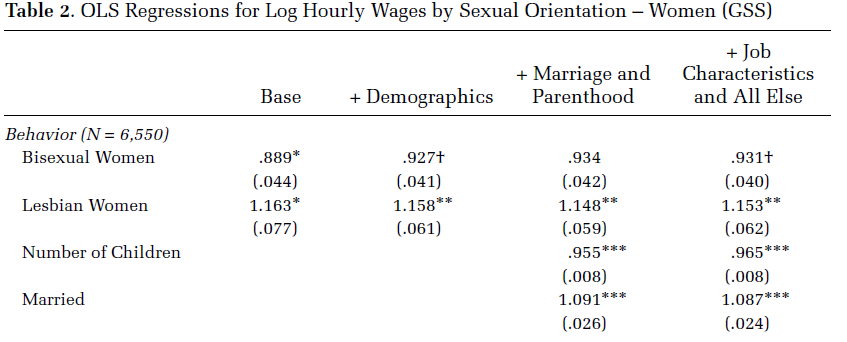
Table 2 shows results of regression models of log wages for women… bisexual women earn 11 percent less than heterosexual women at baseline (eb = .89, p < .05). After accounting for all other factors, bisexual women still earn 7 percent less than comparable heterosexual women, providing support for Hypothesis 6 (eb = .93, p < .10)… Lesbian women earn more than heterosexual women at baseline (eb = 1.16, p < .05). This difference remains significant and substantively similar in size after accounting for all factors (eb = 1.15, p < .01).
* Model from Table 2 of Mize (2016) ASR
usetdm smi_gss, clear
Loading dataset...
(SMI | Mize 2016 ASR | GSS Data on Sexual Behavior and Wages)svy: reg logwages i.partners75 age i.educcat i.race year ///
numchild married i.region4 i.metro parttime i.isco88cat ///
if male==0, eform(Factor)(running regress on estimation sample)
Survey: Linear regression
Number of strata = 1 Number of obs = 6,550
Number of PSUs = 336 Population size = 6,567.8471
Design df = 335
F(26, 310) = 67.90
Prob > F = 0.0000
R-squared = 0.2560
-------------------------------------------------------------------------------
| Linearized
logwages | Factor std. err. t P>|t| [95% conf. interval]
--------------+----------------------------------------------------------------
partners75 |
Bisexual | 0.931 0.040 -1.658 0.098 0.855 1.013
Gay | 1.153 0.062 2.652 0.008 1.037 1.282
|
age | 1.016 0.001 15.741 0.000 1.014 1.018
|
educcat |
high school | 1.389 0.070 6.502 0.000 1.258 1.534
junior col.. | 1.730 0.094 10.032 0.000 1.554 1.926
bachelor | 1.899 0.109 11.201 0.000 1.697 2.126
graduate | 2.445 0.153 14.283 0.000 2.162 2.765
|
race |
black | 1.034 0.032 1.077 0.282 0.973 1.100
other | 0.999 0.054 -0.023 0.982 0.897 1.112
|
year | 0.996 0.002 -2.535 0.012 0.993 0.999
numchild | 0.965 0.008 -4.316 0.000 0.950 0.981
married | 1.087 0.024 3.756 0.000 1.040 1.135
|
region4 |
Midwest | 0.889 0.039 -2.666 0.008 0.815 0.970
South | 0.856 0.038 -3.540 0.000 0.785 0.933
West | 0.979 0.047 -0.439 0.661 0.891 1.076
|
1.metro | 1.050 0.033 1.552 0.122 0.987 1.118
parttime | 0.842 0.024 -6.000 0.000 0.795 0.891
|
isco88cat |
lo control.. | 0.844 0.025 -5.633 0.000 0.795 0.895
routine no.. | 0.659 0.023 -11.957 0.000 0.616 0.706
sempl with.. | 0.717 0.056 -4.252 0.000 0.614 0.836
sempl with.. | 0.557 0.042 -7.763 0.000 0.480 0.646
manual sup.. | 0.916 0.083 -0.963 0.336 0.767 1.095
skilled ma.. | 0.742 0.042 -5.290 0.000 0.665 0.829
semi-unski.. | 0.611 0.025 -12.130 0.000 0.564 0.662
farm labor | 0.572 0.078 -4.071 0.000 0.437 0.749
selfempl f.. | 0.645 0.216 -1.310 0.191 0.334 1.246
|
_cons | 25685.979 86067.823 3.030 0.003 35.251 1.87e+07
-------------------------------------------------------------------------------qui margins, at(age=(20(5)80))
marginsplot, recastci(rline) ciopts(lpat(dash) col(gs14)) ///
title("[2.8.c] Predicted Log Wages by Age (Women Workers Only)") ///
ytitle("Log Wages") ylab(1(0.5)3.5)Variables that uniquely identify margins: age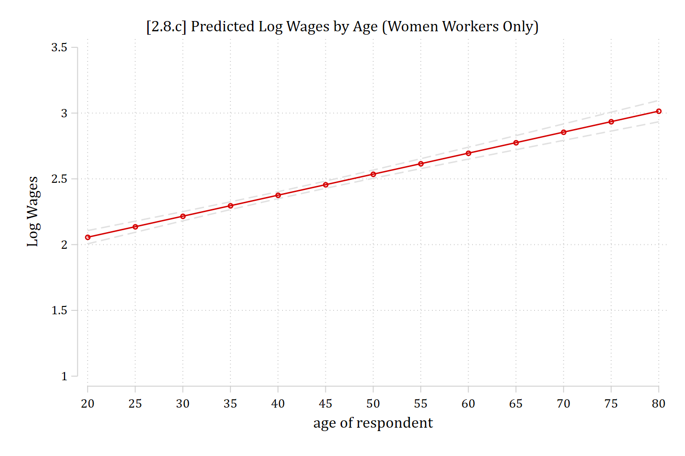
The effect on the log of wages is linear (but how would you interpret log wages?)
Interpretation in the natural metric of the DV
- Logged DV regression models can be very useful; however, you almost certainly do not set out to study effects on the log of wages. Interpreting the factor change coefficients is one useful alternative
- Factor change coefficients are in the natural metric of the DV (a plus), but are multiplicative rather than additive (generally, a negative)
- Focusing on interpreting predictions and marginal effects (which are calculated from the predictions) hold key benefits here as you can convert the prediction back into the natural metric of the DV (in this example, wages) and MEs are additive effects (just like your trusty linear regression coefficients)
- Recall the general formula for a marginal effect:
\[ME = \eta\left( x_{k} = end,\ \mathbf{x}_{- k} = \mathbf{x}^{\mathbf{*}} \right) - \eta\left( x_{k} = start,\ \mathbf{x}_{- k} = \mathbf{x}^{\mathbf{*}} \right)\]
- For our linear regression examples earlier, \(\eta\) (the prediction) was easy to solve for as it was just the result of solving the regression equation for \(\mathbf{x\beta}\)
- This is because our linear regression model coefficients were already in the natural metric of the DV (e.g. occupational prestige)
Converting predictions to natural metric of DV
- For logged DV regression models, fairly straightforward to transform the \(\mathbf{x\beta}\) prediction (which is in \(ln(y)\) metric) back to the natural y metric by exponentiating it*. E.g.
\[\widehat{\ln(wages)} = \mathbf{x\beta}\]
\[\eta = \widehat{wages} = \exp(\mathbf{x\beta})\]
- Note the formula for marginal effects are identical in logged DV regression models as they are in linear models (i.e., the formulas shown earlier in these notes are equally applicable in both types of models)
- The only difference is that the formula for \(\eta\) has changed
- I.e. We are still interpreting effects in terms of differences in predictions; the only thing that has changed is how we get to the prediction (\(\eta\)) of interest
*But note some important complications if you had values <1 in the original metric of the variable
qui margins, at(age=(20(5)80)) expression(exp(predict(xb)))
marginsplot, recastci(rline) ciopts(lpat(dash) col(gs14)) ///
    title("[2.8.d] Predicted Hourly Wages by Age (Women Workers Only)") ///
    ytitle("Hourly Wages") ylab(5(5)30)
Variables that uniquely identify margins: age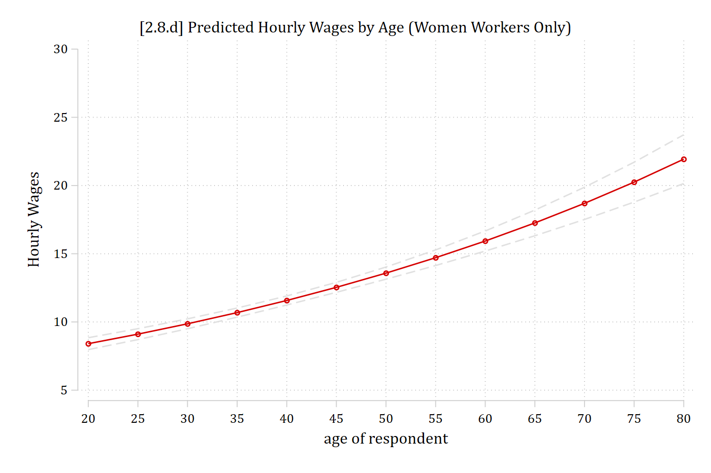
Note the nonlinearities. This is despite no age2 coefficient in the model. The model is inherently nonlinear in the wages metric due to ln(wages) used as the DV
qui margins, at(age=(20(5)80) partners75=(1 2 3)) expression(exp(predict(xb)))
marginsplot, noci title("[2.8.e] Predicted Hourly Wages by Age (Women Workers
Only)") ///
    ytitle("Hourly Wages") ylab(5(5)30)
Variables that uniquely identify margins: age partners75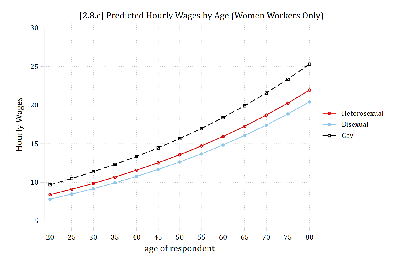
*Note the interaction effect (e.g. size of sexuality gaps vary at different ages) despite no interaction terms in model. Nonlinearities produce interaction effect
What happens when we add age2 to the model? Even more nonlinearities and interaction effects. Just as in linear regression, in loglinear regression the polynomial allows for the slope of the prediction line to change at some point. Here the effect reverses at higher ages.
svy: reg logwages i.partners75##c.age##c.age i.educcat i.race year ///
    numchild married i.region4 i.metro parttime i.isco88cat ///
    if male==0, eform(Factor)
(running regress on estimation sample)
Survey: Linear regression
Number of strata = 1 Number of obs = 6,550
Number of PSUs = 336 Population size = 6,567.8471
Design df = 335
F(31, 305) = 61.30
Prob > F = 0.0000
R-squared = 0.2715
-------------------------------------------------------------------------------
| Linearized
logwages | Factor std. err. t P>|t| [95% conf. interval]
--------------+----------------------------------------------------------------
partners75 |
Bisexual | 0.644 0.386 -0.734 0.463 0.198 2.094
Gay | 1.388 0.837 0.543 0.587 0.424 4.548
|
age | 1.073 0.006 12.347 0.000 1.061 1.085
|
partners75#|
c.age |
Bisexual | 1.020 0.032 0.634 0.526 0.960 1.084
Gay | 0.988 0.028 -0.438 0.662 0.934 1.045
|
c.age#c.age | 0.999 0.000 -9.638 0.000 0.999 1.000
|
partners75#|
c.age#c.age |
Bisexual | 1.000 0.000 -0.678 0.498 0.999 1.000
Gay | 1.000 0.000 0.534 0.594 1.000 1.001
|
educcat |
high school | 1.350 0.067 6.099 0.000 1.226 1.488
junior col.. | 1.639 0.088 9.218 0.000 1.475 1.821
bachelor | 1.808 0.102 10.446 0.000 1.617 2.021
graduate | 2.313 0.144 13.496 0.000 2.047 2.614
|
race |
black | 1.020 0.031 0.639 0.524 0.960 1.083
other | 0.996 0.054 -0.078 0.938 0.896 1.107
|
year | 0.997 0.002 -1.768 0.078 0.994 1.000
numchild | 0.954 0.008 -5.793 0.000 0.939 0.970
married | 1.045 0.022 2.047 0.041 1.002 1.089
|
region4 |
Midwest | 0.896 0.038 -2.574 0.010 0.824 0.974
South | 0.864 0.037 -3.398 0.001 0.794 0.940
West | 0.972 0.045 -0.602 0.548 0.887 1.066
|
1.metro | 1.057 0.033 1.765 0.078 0.994 1.124
parttime | 0.884 0.025 -4.327 0.000 0.836 0.935
|
isco88cat |
lo control.. | 0.845 0.025 -5.637 0.000 0.796 0.896
routine no.. | 0.666 0.023 -11.812 0.000 0.623 0.713
sempl with.. | 0.724 0.056 -4.142 0.000 0.621 0.844
sempl with.. | 0.549 0.041 -8.053 0.000 0.475 0.636
manual sup.. | 0.922 0.080 -0.929 0.354 0.778 1.094
skilled ma.. | 0.745 0.041 -5.339 0.000 0.668 0.830
semi-unski.. | 0.617 0.025 -11.920 0.000 0.570 0.668
farm labor | 0.581 0.077 -4.102 0.000 0.448 0.754
selfempl f.. | 0.644 0.221 -1.281 0.201 0.328 1.266
|
_cons | 671.048 2236.546 1.953 0.052 0.954 4.72e+05
-------------------------------------------------------------------------------est store smimod
qui margins, at(age=(20(5)80) partners75=(1 2 3)) expression(exp(predict(xb)))
marginsplot, noci title("[2.8.f] Predicted Hourly Wages by Age (Women Workers
Only)") ///
ytitle("Hourly Wages") ylab(0(5)25)Variables that uniquely identify margins: age partners75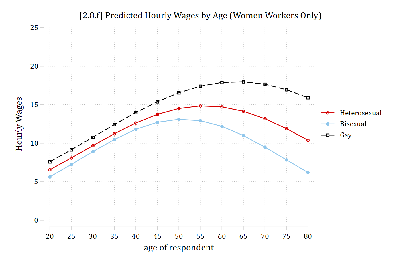
Logged DV regression models—marginal effects
- The coefficients are no longer directly interpretable when we have quadratic and/or interaction terms as we do for the model presented in the plot above
- Marginal effects can still provide an overall summary for the effects of interest—for this example, the effect of sexual identity for women
- Remember to exponentiate the predictions when you calculate the MEs so you are in the wage metric instead of the ln(wage) metric [which will be the default]
est restore smimod(results smimod are active now)mchange partners75, expression(exp(predict(xb)))svy regress: Changes in Margin | Number of obs = 6550
Expression: , exp(predict(xb))
| Change p-value
--------------------------+---------------------
partners75 |
Bisexual vs Heterosexual | -1.191 0.017
Gay vs Heterosexual | 1.676 0.019
Gay vs Bisexual | 2.867 0.001
Average prediction
11.998 Bisexual women earn about $1.19 less an hour than heterosexual women
On average, lesbian women earn about $1.68 more per hour than heterosexual women and about $2.87 more than bisexual women
- These interpretations are useful and straightforward summaries of the effect of sexual identity—despite the rather complicated model that produced them
- I would include these and the plot above. Probably start with the overall effects (MEs) and then move on to the complications (plot)