4.1 Multinomial Logit Model

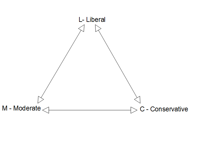
Multinomial logit with three outcomes

Categories L, M, and C with nL, nM, and nC observations in each category

Triangle diagram with L - Liberal at the top and M - Moderate and C - Conservative at the bottom corners; a two-headed arrow connects each pair of outcomes.

use "https://tdmize.github.io/data/data/cda_gss", clear
(cda_gss.dta |  GSS 1972-2021 CDA - Categorical Data Analysis | date created 202
> 3)
keep if year >= 2016 & year <= 2021
(59,599 observations deleted)
drop if missing(conserv, age, woman, race3, college, married, parent, faminc)
(1,421 observations deleted)
fre polviews3
polviews3 -- Political View Categories
--------------------------------------------------------------------
                       |      Freq.    Percent      Valid       Cum.
-----------------------+--------------------------------------------
Valid   1 Liberal      |       2492      31.84      31.84      31.84
        2 Moderate     |       2791      35.66      35.66      67.51
        3 Conservative |       2543      32.49      32.49     100.00
        Total          |       7826     100.00     100.00           
--------------------------------------------------------------------
library(haven)           # import Stata data and labels
library(dplyr)           # data manipulation
library(sjmisc)          # frq() frequency tables
library(nnet)            # multinomial logit: multinom()
library(marginaleffects) # hypothesis tests
library(car)             # Anova()

gss <- read_dta("https://tdmize.github.io/data/data/cda_gss.dta")

gss <- gss |> filter(year >= 2016 & year <= 2021)

# Keep model variables; drop any missing data
gss <- gss[c("polviews3", "age", "woman", "race3", "college", "married", "parent",
  "faminc", "employed", "conserv")]
gss <- gss[complete.cases(gss[c("conserv", "age", "woman", "race3", "college",
  "married", "parent", "faminc")]), ]

frq(gss$polviews3)
Political View Categories (x) <numeric> 
# total N=7826 valid N=7826 mean=2.01 sd=0.80

Value |        Label |    N | Raw % | Valid % | Cum. %
------------------------------------------------------
    1 |      Liberal | 2492 | 31.84 |   31.84 |  31.84
    2 |     Moderate | 2791 | 35.66 |   35.66 |  67.51
    3 | Conservative | 2543 | 32.49 |   32.49 | 100.00
 <NA> |         <NA> |    0 |  0.00 |    <NA> |   <NA>
# Treat binary/nominal variables as factors
gss <- gss |>
  mutate(across(c(polviews3, woman, race3, college, married, parent, employed), as_factor)) |>
  droplevels()

Multinomial logit is a set of binary logits that are simultaneously estimated

  • L vs M using nL + nM observations

    \[\ln\left[\frac{\Pr(L\,|\,\mathbf{x}_{i})}{\Pr(M\,|\,\mathbf{x}_{i})}\right] = \beta_{0,L|M} + \boldsymbol{\beta}_{X,L|M}\,\mathbf{x}_{i}\]

    • Where xi includes all focal IVs and control variables in the model
  • M vs C using nM + nC observations

\[\ln\left[\frac{\Pr(M\,|\,\mathbf{x}_{i})}{\Pr(C\,|\,\mathbf{x}_{i})}\right] = \beta_{0,M|C} + \boldsymbol{\beta}_{X,M|C}\,\mathbf{x}_{i}\]

  • L vs C using nL + nC observations

\[\ln\left[\frac{\Pr(L\,|\,\mathbf{x}_{i})}{\Pr(C\,|\,\mathbf{x}_{i})}\right] = \beta_{0,L|C} + \boldsymbol{\beta}_{X,L|C}\,\mathbf{x}_{i}\]

Minimal sets of coefficient estimates

  • Because of mathematical links among odds, some coefficients are “extra”
    • \(\beta_{L|M} = \beta_{L|C} + \beta_{C|M}\)
    • From any two of L/M, L/C, and C/M, you can compute the third
  • With J outcome categories you only need J - 1 comparisons/sets of coefficients
  • Each set of J - 1 comparisons is a minimal set
    • Different software computes different minimal sets
  • In Stata, use the mlogit command
    • Default base/reference outcome category is one with most observations
    • Change base/reference category with base(#) option
mlogit …, base(3)
  • In R, use the multinom function in the nnet package
    • Default base/reference outcome category is first one
    • To change base/reference category, need to change the reference level in the variable itself before fitting model using relevel
gss$polviews3 <- relevel(gss$polviews3, ref = "Moderate")

multinom(polviews3 ~ age + woman + race3 …, data = gss)

mlogit estimates a minimal set of coefficients

mlogit polviews3 c.age i.woman i.race3 i.college ///
    i.married i.parent c.faminc i.employed
Iteration 0:  Log likelihood = -8584.7295  
Iteration 1:  Log likelihood = -8197.0737  
Iteration 2:  Log likelihood = -8195.2338  
Iteration 3:  Log likelihood = -8195.2335  

Multinomial logistic regression                         Number of obs =  7,823
                                                        LR chi2(18)   = 778.99
                                                        Prob > chi2   = 0.0000
Log likelihood = -8195.2335                             Pseudo R2     = 0.0454

-------------------------------------------------------------------------------
    polviews3 | Coefficient  Std. err.      z    P>|z|     [95% conf. interval]
--------------+----------------------------------------------------------------
Liberal       |
          age |      0.001      0.002    0.518   0.604       -0.003       0.005
              |
        woman |
       Women  |     -0.004      0.058   -0.065   0.948       -0.118       0.110
              |
        race3 |
       black  |      0.014      0.080    0.175   0.861       -0.143       0.171
       other  |      0.003      0.095    0.029   0.977       -0.183       0.189
              |
      college |
College De..  |      0.902      0.064   14.071   0.000        0.776       1.028
              |
      married |
     Married  |     -0.084      0.065   -1.298   0.194       -0.211       0.043
              |
       parent |
      Parent  |     -0.519      0.069   -7.476   0.000       -0.655      -0.383
       faminc |      0.004      0.001    3.746   0.000        0.002       0.005
              |
     employed |
         Yes  |     -0.063      0.064   -0.995   0.320       -0.188       0.061
        _cons |     -0.219      0.121   -1.816   0.069       -0.456       0.017
--------------+----------------------------------------------------------------
Moderate      |  (base outcome)
--------------+----------------------------------------------------------------
Conservative  |
          age |      0.014      0.002    7.329   0.000        0.010       0.018
              |
        woman |
       Women  |     -0.272      0.057   -4.770   0.000       -0.384      -0.160
              |
        race3 |
       black  |     -0.596      0.087   -6.822   0.000       -0.767      -0.424
       other  |     -0.405      0.101   -4.011   0.000       -0.603      -0.207
              |
      college |
College De..  |      0.171      0.066    2.602   0.009        0.042       0.299
              |
      married |
     Married  |      0.275      0.062    4.410   0.000        0.153       0.397
              |
       parent |
      Parent  |      0.105      0.073    1.433   0.152       -0.039       0.249
       faminc |      0.001      0.001    1.505   0.132       -0.000       0.003
              |
     employed |
         Yes  |      0.119      0.064    1.867   0.062       -0.006       0.243
        _cons |     -0.935      0.127   -7.365   0.000       -1.184      -0.686
-------------------------------------------------------------------------------
est store pol3mod
# Moderate as the base/reference category (Stata's default here)
gss$polviews3 <- relevel(gss$polviews3, ref = "Moderate")

pol3mod <- multinom(polviews3 ~ age + woman + race3 + college + married + parent +
  faminc + employed, data = gss, trace = FALSE)
summary(pol3mod)
Call:
multinom(formula = polviews3 ~ age + woman + race3 + college + 
    married + parent + faminc + employed, data = gss, trace = FALSE)

Coefficients:
             (Intercept)          age   womanWomen  race3black   race3other collegeCollege Degree
Liberal       -0.2194806 0.0009917368 -0.003769701  0.01402515  0.002759557              0.901998
Conservative  -0.9354447 0.0139484020 -0.272207692 -0.59553752 -0.405149847              0.170826
             marriedMarried parentParent      faminc employedYes
Liberal         -0.08398208   -0.5186556 0.003529939  -0.0633015
Conservative     0.27489769    0.1052532 0.001451543   0.1186752

Std. Errors:
             (Intercept)         age womanWomen race3black race3other collegeCollege Degree
Liberal        0.1208599 0.001913642 0.05821723 0.08001720 0.09495155            0.06410471
Conservative   0.1270174 0.001903207 0.05707173 0.08729248 0.10101386            0.06564945
             marriedMarried parentParent       faminc employedYes
Liberal          0.06471308   0.06937451 0.0009422861  0.06362598
Conservative     0.06233462   0.07343414 0.0009647622  0.06357645

Residual Deviance: 16390.47 
AIC: 16430.47 

Minimal sets vs all possible contrasts

  • Do not judge statistical significance using tests from a minimal set (which is what Stata and R produce by default)
  • Calculating all coefficients for all contrasts yourself is cumbersome. The spost13 command listcoef in Stata will do this for you*
    • Wrapping your head around this many coefficients/contrasts is difficult:
listcoef, help
mlogit (N=7823): Factor change in the odds of polviews3 

Variable: age (sd=17.361)
------------------------------------------------------------------------------
                             |         b        z    P>|z|       e^b   e^bStdX
-----------------------------+------------------------------------------------
Liberal      vs Moderate     |    0.0010    0.518    0.604     1.001     1.017
Liberal      vs Conservative |   -0.0130   -6.489    0.000     0.987     0.799
Moderate     vs Liberal      |   -0.0010   -0.518    0.604     0.999     0.983
Moderate     vs Conservative |   -0.0139   -7.329    0.000     0.986     0.785
Conservative vs Liberal      |    0.0130    6.489    0.000     1.013     1.252
Conservative vs Moderate     |    0.0139    7.329    0.000     1.014     1.274
------------------------------------------------------------------------------

Variable: 1.woman (sd=0.498)
------------------------------------------------------------------------------
                             |         b        z    P>|z|       e^b   e^bStdX
-----------------------------+------------------------------------------------
Liberal      vs Moderate     |   -0.0038   -0.065    0.948     0.996     0.998
Liberal      vs Conservative |    0.2684    4.515    0.000     1.308     1.143
Moderate     vs Liberal      |    0.0038    0.065    0.948     1.004     1.002
Moderate     vs Conservative |    0.2722    4.770    0.000     1.313     1.145
Conservative vs Liberal      |   -0.2684   -4.515    0.000     0.765     0.875
Conservative vs Moderate     |   -0.2722   -4.770    0.000     0.762     0.873
------------------------------------------------------------------------------

Variable: 2.race3 (sd=0.349)
------------------------------------------------------------------------------
                             |         b        z    P>|z|       e^b   e^bStdX
-----------------------------+------------------------------------------------
Liberal      vs Moderate     |    0.0140    0.175    0.861     1.014     1.005
Liberal      vs Conservative |    0.6096    6.581    0.000     1.840     1.237
Moderate     vs Liberal      |   -0.0140   -0.175    0.861     0.986     0.995
Moderate     vs Conservative |    0.5955    6.822    0.000     1.814     1.231
Conservative vs Liberal      |   -0.6096   -6.581    0.000     0.544     0.808
Conservative vs Moderate     |   -0.5955   -6.822    0.000     0.551     0.812
------------------------------------------------------------------------------

Variable: 3.race3 (sd=0.292)
------------------------------------------------------------------------------
                             |         b        z    P>|z|       e^b   e^bStdX
-----------------------------+------------------------------------------------
Liberal      vs Moderate     |    0.0028    0.029    0.977     1.003     1.001
Liberal      vs Conservative |    0.4079    3.872    0.000     1.504     1.126
Moderate     vs Liberal      |   -0.0028   -0.029    0.977     0.997     0.999
Moderate     vs Conservative |    0.4051    4.011    0.000     1.500     1.125
Conservative vs Liberal      |   -0.4079   -3.872    0.000     0.665     0.888
Conservative vs Moderate     |   -0.4051   -4.011    0.000     0.667     0.889
------------------------------------------------------------------------------

Variable: 1.college (sd=0.485)
------------------------------------------------------------------------------
                             |         b        z    P>|z|       e^b   e^bStdX
-----------------------------+------------------------------------------------
Liberal      vs Moderate     |    0.9020   14.071    0.000     2.465     1.549
Liberal      vs Conservative |    0.7312   11.234    0.000     2.078     1.426
Moderate     vs Liberal      |   -0.9020  -14.071    0.000     0.406     0.645
Moderate     vs Conservative |   -0.1708   -2.602    0.009     0.843     0.920
Conservative vs Liberal      |   -0.7312  -11.234    0.000     0.481     0.701
Conservative vs Moderate     |    0.1708    2.602    0.009     1.186     1.086
------------------------------------------------------------------------------

Variable: 1.married (sd=0.498)
------------------------------------------------------------------------------
                             |         b        z    P>|z|       e^b   e^bStdX
-----------------------------+------------------------------------------------
Liberal      vs Moderate     |   -0.0840   -1.298    0.194     0.919     0.959
Liberal      vs Conservative |   -0.3589   -5.454    0.000     0.698     0.836
Moderate     vs Liberal      |    0.0840    1.298    0.194     1.088     1.043
Moderate     vs Conservative |   -0.2749   -4.410    0.000     0.760     0.872
Conservative vs Liberal      |    0.3589    5.454    0.000     1.432     1.196
Conservative vs Moderate     |    0.2749    4.410    0.000     1.316     1.147
------------------------------------------------------------------------------

Variable: 1.parent (sd=0.450)
------------------------------------------------------------------------------
                             |         b        z    P>|z|       e^b   e^bStdX
-----------------------------+------------------------------------------------
Liberal      vs Moderate     |   -0.5187   -7.476    0.000     0.595     0.792
Liberal      vs Conservative |   -0.6239   -8.543    0.000     0.536     0.755
Moderate     vs Liberal      |    0.5187    7.476    0.000     1.680     1.263
Moderate     vs Conservative |   -0.1053   -1.433    0.152     0.900     0.954
Conservative vs Liberal      |    0.6239    8.543    0.000     1.866     1.324
Conservative vs Moderate     |    0.1053    1.433    0.152     1.111     1.048
------------------------------------------------------------------------------

Variable: faminc (sd=35.539)
------------------------------------------------------------------------------
                             |         b        z    P>|z|       e^b   e^bStdX
-----------------------------+------------------------------------------------
Liberal      vs Moderate     |    0.0035    3.746    0.000     1.004     1.134
Liberal      vs Conservative |    0.0021    2.275    0.023     1.002     1.077
Moderate     vs Liberal      |   -0.0035   -3.746    0.000     0.996     0.882
Moderate     vs Conservative |   -0.0015   -1.505    0.132     0.999     0.950
Conservative vs Liberal      |   -0.0021   -2.275    0.023     0.998     0.929
Conservative vs Moderate     |    0.0015    1.505    0.132     1.001     1.053
------------------------------------------------------------------------------

Variable: 1.employed (sd=0.493)
------------------------------------------------------------------------------
                             |         b        z    P>|z|       e^b   e^bStdX
-----------------------------+------------------------------------------------
Liberal      vs Moderate     |   -0.0633   -0.995    0.320     0.939     0.969
Liberal      vs Conservative |   -0.1820   -2.730    0.006     0.834     0.914
Moderate     vs Liberal      |    0.0633    0.995    0.320     1.065     1.032
Moderate     vs Conservative |   -0.1187   -1.867    0.062     0.888     0.943
Conservative vs Liberal      |    0.1820    2.730    0.006     1.200     1.094
Conservative vs Moderate     |    0.1187    1.867    0.062     1.126     1.060
------------------------------------------------------------------------------
       b = raw coefficient
       z = z-score for test of b=0
   P>|z| = p-value for z-test
     e^b = exp(b) = factor change in odds for unit increase in X
 e^bStdX = exp(b*SD of X) = change in odds for SD increase in X
# All contrasts among the outcomes: refit the model with each outcome
# category as the base/reference category
all_contrasts <- function(model, term) {
  data <- eval(model$call$data)
  y <- all.vars(formula(model))[1]
  out <- lapply(model$lev, function(ref) {
    data[[y]] <- relevel(data[[y]], ref = ref)
    s <- summary(update(model, data = data))
    b <- s$coefficients[, term]
    z <- b / s$standard.errors[, term]
    data.frame(contrast = paste(rownames(s$coefficients), "vs", ref),
      b = round(b, 4), z = round(z, 3), p = round(2 * pnorm(-abs(z)), 3),
      exp_b = round(exp(b), 3), row.names = NULL)
  })
  do.call(rbind, out)
}

all_contrasts(pol3mod, "age")
                  contrast       b      z     p exp_b
1      Liberal vs Moderate  0.0010  0.518 0.604 1.001
2 Conservative vs Moderate  0.0139  7.329 0.000 1.014
3      Moderate vs Liberal -0.0010 -0.518 0.604 0.999
4  Conservative vs Liberal  0.0130  6.489 0.000 1.013
5 Moderate vs Conservative -0.0139 -7.329 0.000 0.986
6  Liberal vs Conservative -0.0130 -6.489 0.000 0.987
all_contrasts(pol3mod, "womanWomen")
                  contrast       b      z     p exp_b
1      Liberal vs Moderate -0.0038 -0.065 0.948 0.996
2 Conservative vs Moderate -0.2722 -4.770 0.000 0.762
3      Moderate vs Liberal  0.0038  0.065 0.948 1.004
4  Conservative vs Liberal -0.2684 -4.515 0.000 0.765
5 Moderate vs Conservative  0.2722  4.770 0.000 1.313
6  Liberal vs Conservative  0.2684  4.515 0.000 1.308
all_contrasts(pol3mod, "race3black")
                  contrast       b      z     p exp_b
1      Liberal vs Moderate  0.0140  0.175 0.861 1.014
2 Conservative vs Moderate -0.5955 -6.822 0.000 0.551
3      Moderate vs Liberal -0.0140 -0.175 0.861 0.986
4  Conservative vs Liberal -0.6096 -6.581 0.000 0.544
5 Moderate vs Conservative  0.5955  6.822 0.000 1.814
6  Liberal vs Conservative  0.6096  6.581 0.000 1.840

*I don’t know of an easy way to automate this in R

  • You don’t want to interpret all of these possible contrasts in order to determine whether your independent variable of interest has an overall effect or not

Testing that a variable has no overall effect

  • The hypothesis that xk has no effect involves a joint test of all J - 1 coefficients for a given IV. E.g., Consider the null hypothesis that age has no overall effect on political views; with 3 outcome categories this is a joint test of 2 age coefficients:

\[H_{0}: \beta_{age,L|M} = \beta_{age,C|M} = 0\]

  • We can use either Wald or likelihood-ratio tests (details on these in the Testing & Fit section of the class). Consider the Wald test:
test [Liberal]age [Conservative]age
 ( 1)  [Liberal]age = 0
 ( 2)  [Conservative]age = 0

           chi2(  2) =   63.56
         Prob > chi2 =    0.0000
hypotheses(pol3mod, joint = c("Liberal:age", "Conservative:age"), joint_test = "chisq")


Joint hypothesis test:
Liberal:age = 0
Conservative:age = 0
 
 ChiSq Pr(>|ChiSq|) Df
  63.6       <0.001  2

Age has a significant effect on political views (p < 0.001)

In Stata, the spost13 command mlogtest will calculate joint tests for all IVs

In R use Anova(modname, type = 2)

mlogtest
Wald tests for independent variables (N=7823)

  Ho: All coefficients associated with given variable(s) are 0

                 |      chi2    df   P>chi2
-----------------+-------------------------
             age |    63.564     2    0.000
         1.woman |    28.775     2    0.000
         2.race3 |    56.007     2    0.000
         3.race3 |    19.721     2    0.000
       1.college |   223.593     2    0.000
       1.married |    33.705     2    0.000
        1.parent |    88.415     2    0.000
          faminc |    14.420     2    0.001
      1.employed |     7.716     2    0.021
# Likelihood-ratio tests (race3 is tested as one variable)
Anova(pol3mod, type = 2)
Analysis of Deviance Table (Type II tests)

Response: polviews3
         LR Chisq Df Pr(>Chisq)    
age        64.311  2  1.084e-14 ***
woman      28.789  2  5.604e-07 ***
race3      72.314  4  7.365e-15 ***
college   225.755  2  < 2.2e-16 ***
married    33.718  2  4.767e-08 ***
parent     87.977  2  < 2.2e-16 ***
faminc     14.462  2  0.0007236 ***
employed    7.748  2  0.0207786 *  
---
Signif. codes:  0 '***' 0.001 '**' 0.01 '*' 0.05 '.' 0.1 ' ' 1

Example interpretations:

- Whether someone has a college degree or not has a significant effect on political views (p < 0.001)

- Gender has a significant overall effect on political views (p < 0.001)

Back to top