The negative binomial model produces higher Pr(y = 0) compared to the Poisson model due to the overdispersion parameter
But, Poisson and negative binomial can struggle with DVs that are ≈ ≥ 50% zeroes because they assume every observation has a positive probability of > 0
E.g., Everyone has a non-zero chance of drinking alcohol; of having at least one depressive symptom; of smoking a cigarette; etc.
In zero inflated models we assume:
Zeroes can occur by multiple processes:
Some people always have 0 counts; some might have 0 counts
This leads to a greater proportion of 0s since they occur two ways
We say “the zeros are inflated”
Positive counts (i.e., > 0) are generated by one process just like Poisson or negative binomial
Zero-inflated models can be motivated theoretically (interested in both the zero or not process as well as the count process) or by necessity of a DV with high proportion of zeroes
The with zeros model: didactically useful
Zeroes occur through two processes
Group A: People who always have 0 counts
Group S: People who sometimes have 0s, but sometimes not
Next, we predict the counts but only for people with observed counts
That is, we do not include observed zeroes in this step
However, some people who were observed with >0 counts are sometimes zero so would not always have counts (e.g., we asked them about # of drinks last month right after the holidays)
Therefore, take the Pr(sometimes zero) into account when predicting counts
The predictions in zero-inflated models are effectively weighted by the probability of not being an always zero
For those we generally think are always zeros (Pr(Always) = 1; Pr(Sometimes) = 0), we give them almost no weight in the calculations of the counts
For those who are very unlikely to be an always a zero (i.e., usually have a non-zero count), we give the most weight
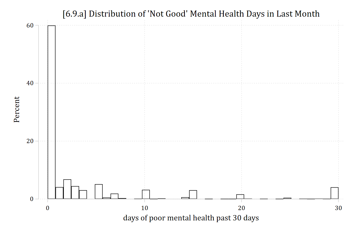
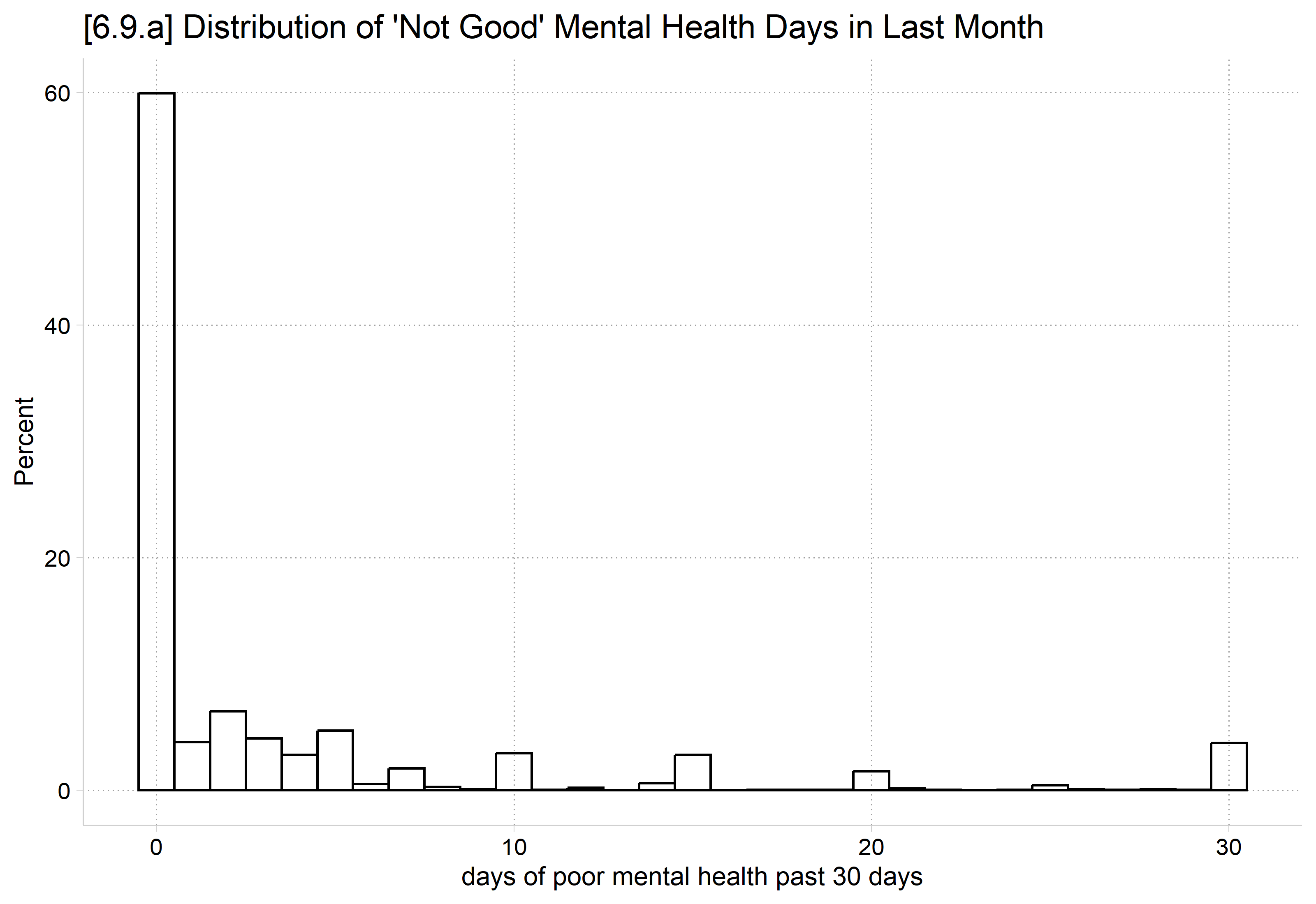
Example: Days in last month of “not good” mental health
GSS (2002, 2006, 2010, 2014)
DV: “Now thinking about your mental health, which includes stress, depression, and problems with emotions, for how many days during the past 30 days was your mental health not good?”
Happily (get it?) this measure has an excess of zeroes
≈ 60% of the sample reports zero days of ‘not good’ mental health
IVs: Gender, income, age, marital status
Controls: Race, education, religiosity, survey year
*6.9.ahist mntlhlth, percent fcolor(none) ///title("[6.9.a] Distribution of 'Not Good' Mental Health Days in Last Month")
(bin=37, start=0, width=.81081081)
library(haven) # import Stata data and labelslibrary(dplyr) # data manipulationlibrary(ggplot2) # graphslibrary(cleanplots) # graph schemecleanplots_defaults()gss <-read_dta("https://tdmize.github.io/data/data/cda_gss.dta")gss <- gss |>filter(year >=2002& year <=2014)# Data management: Christian (Protestant, Catholic, Christian) vs not religiousgss <- gss |>mutate(notrelig =case_when(relig %in%c(1, 2, 11) ~0, relig ==4~1))gss <- gss[complete.cases(gss[c("mntlhlth", "physhlth", "woman", "race3", "year","college", "parent", "faminc", "metro", "notrelig", "married")]), ]# 6.9.aggplot(gss, aes(x = mntlhlth)) +geom_histogram(aes(y =after_stat(100* count /sum(count))), binwidth =1,fill =NA, color ="black") +labs(title ="[6.9.a] Distribution of 'Not Good' Mental Health Days in Last Month",x ="days of poor mental health past 30 days", y ="Percent")