Appendix 3D: Distribution of Marginal Effects

• Recall that an average marginal effect (AME) is the mean (average) of separate marginal effects calculated for each observation
  • The difference between two predictions for each observation indicates the effect for that specific observation (ME_i)

\[{ME}_{i} = \eta(x_{k} = {end}_{i}, \mathbf{x}_{-k} = \mathbf{x}_{-k,i}) - \eta(x_{k} = {start}_{i}, \mathbf{x}_{-k} = \mathbf{x}_{-k,i})\]

• Effects will vary for each observation because start and end values will differ (e.g., \({start}_{i}\) = your current age; \({end}_{i}\) could be your current age + 1) and the models are inherently nonlinear
• Effects will also vary because value of control variables (\(\mathbf{x}_{-k,i}\)) will also differ for each observation and the models are inherently interactive
• The average marginal effect (AME) averages these effects over all observations in the data:

\[AME = \frac{1}{N}\sum_{i = 1}^{N}\left\{\eta(x_{k} = {end}_{i}, \mathbf{x}_{-k} = \mathbf{x}_{-k,i}) - \eta(x_{k} = {start}_{i}, \mathbf{x}_{-k} = \mathbf{x}_{-k,i})\right\}\]

Examining distributions of MEs

• Averages do not indicate variation in the sample.
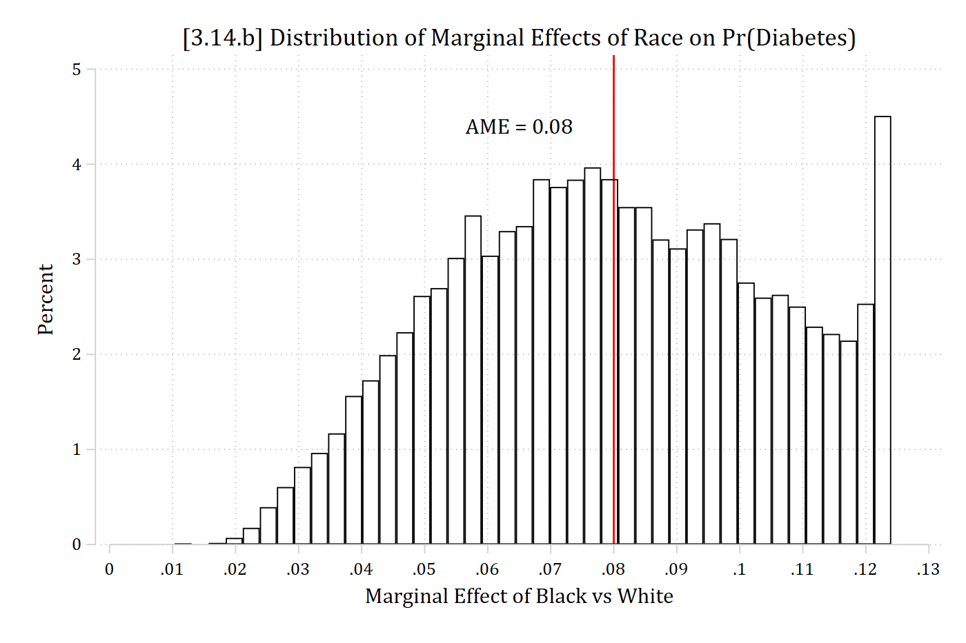
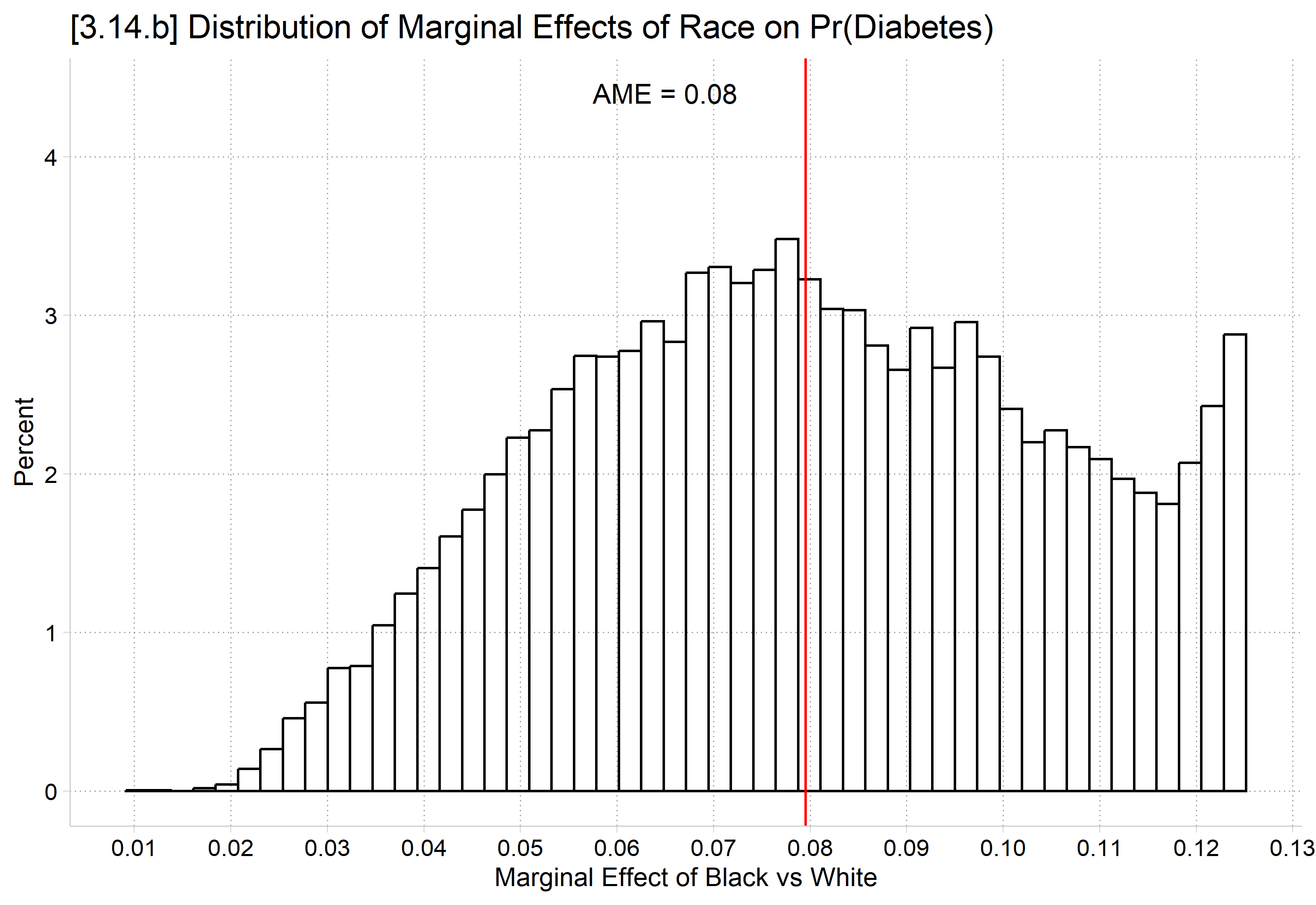
  • E.g., Racial differences might depend on the levels of other variables
    • We already know from our marginsplot that the effect of BMI is different across the range of BMI—which means it varies for different people as people have different BMIs (due to nonlinearities in the effect of BMI)
    • Effect of BMI might also depend on other factors accounted for in the model (e.g., for men vs women; for people of different ages; etc.)
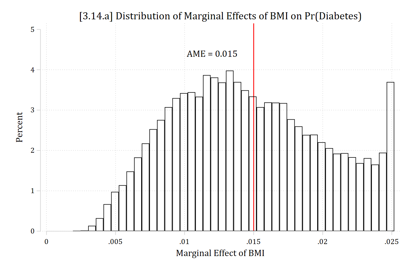
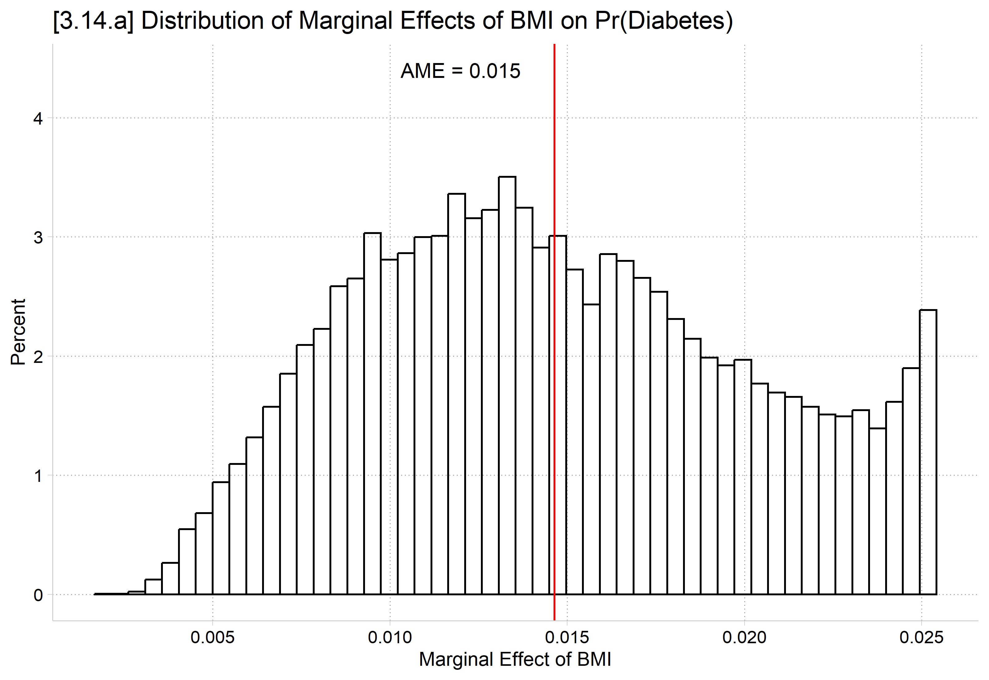
• This suggests the importance of looking at the distribution of marginal effects
• This is not commonly done, but should be (and is now easy to do in Stata 14+)
  • See Appendix 3A for details

Stata

use "https://tdmize.github.io/data/data/hrs06", clear

(hrs06_dmv.dta | Health & Retirement Study 2006 | DMV Workshop)

qui logit diabetes c.age i.black c.bmi i.woman i.ed4cat, or
est store diabmod
* Distribution of marginal effects (AMEs)
margins, dydx(black) gen(MEs_black)

Average marginal effects                                Number of obs = 17,012
Model VCE: OIM

Expression: Pr(diabetes), predict()
dy/dx wrt:  1.black

------------------------------------------------------------------------------
             |            Delta-method
             |      dy/dx   std. err.      z    P>|z|     [95% conf. interval]
-------------+----------------------------------------------------------------
       black |
      Black  |      0.080      0.009    8.862   0.000        0.062       0.097
------------------------------------------------------------------------------
Note: dy/dx for factor levels is the discrete change from the base level.

margins, dydx(bmi) gen(MEs_bmi)

Average marginal effects                                Number of obs = 17,012
Model VCE: OIM

Expression: Pr(diabetes), predict()
dy/dx wrt:  bmi

------------------------------------------------------------------------------
             |            Delta-method
             |      dy/dx   std. err.      z    P>|z|     [95% conf. interval]
-------------+----------------------------------------------------------------
         bmi |      0.015      0.000   31.128   0.000        0.014       0.016
------------------------------------------------------------------------------

hist MEs_bmi, percent fcolor(none) ylabel(0(1)5) ///
    xline(.015, lcolor(red) lstyle(solid)) ///
    text(4.4 .012 "AME = 0.015") xtitle("Marginal Effect of BMI") ///
    title("[3.14.a] Distribution of Marginal Effects of BMI on Pr(Diabetes)")

(bin=42, start=.0019094, width=.00055405)

R

library(haven)           # import Stata data and labels
library(dplyr)           # data manipulation
library(ggplot2)         # graphs
library(marginaleffects) # predictions and marginal effects
library(cleanplots)      # graph scheme
cleanplots_defaults()

hrs <- read_dta("https://tdmize.github.io/data/data/hrs06.dta")

# Treat binary/nominal variables as factors using their value labels
hrs <- hrs |>
  mutate(black = as_factor(black), woman = as_factor(woman), ed4cat = as_factor(ed4cat))

diabmod <- glm(diabetes ~ age + black + bmi + woman + ed4cat,
  family = binomial(link = "logit"), data = hrs)

# Marginal effects for every observation
MEs_black <- comparisons(diabmod, variables = "black")
MEs_bmi <- slopes(diabmod, variables = "bmi")

ggplot(MEs_bmi, aes(x = estimate)) +
  geom_histogram(aes(y = after_stat(100 * count / sum(count))), bins = 50,
    fill = NA, color = "black") +
  geom_vline(xintercept = mean(MEs_bmi$estimate), color = "red") +
  annotate("text", x = .012, y = 4.4, label = "AME = 0.015") +
  labs(title = "[3.14.a] Distribution of Marginal Effects of BMI on Pr(Diabetes)",
    x = "Marginal Effect of BMI", y = "Percent")

Stata

hist MEs_black2, percent xlabel(0(.01).13) fcolor(none) ylabel(0(1)5) ///
    xline(.08, lcolor(red) lstyle(solid)) ///
    text(4.4 .065 "AME = 0.08") xtitle("Marginal Effect of Black vs White") //
/
    title("[3.14.b] Distribution of Marginal Effects of Race on Pr(Diabetes)")

(bin=42, start=.01030588, width=.00270743)

R

ggplot(MEs_black, aes(x = estimate)) +
  geom_histogram(aes(y = after_stat(100 * count / sum(count))), bins = 50,
    fill = NA, color = "black") +
  geom_vline(xintercept = mean(MEs_black$estimate), color = "red") +
  annotate("text", x = .065, y = 4.4, label = "AME = 0.08") +
  scale_x_continuous(breaks = seq(0, .13, .01)) +
  labs(title = "[3.14.b] Distribution of Marginal Effects of Race on Pr(Diabetes)",
    x = "Marginal Effect of Black vs White", y = "Percent")

Comparison of distribution of marginal effects in linear and nonlinear models

• What would you expect the distribution of marginal effects to look like if the model was linear and additive?
• Consider BMI as the dependent variable now with two different specifications:
  • Continuous BMI (≈ 10 – 83)
  • Binary: “low or medium BMI=0” vs. “high BMI=1”
• Our focal IVs are age and gender (coded as woman=1)
  • Also controlling for race and education

Stata

// Comparison of AMEs in OLS and Logit
drop if missing(bmi, age, black, woman, ed4cat)

(507 observations deleted)

gen highbmi = bmicat
lab var highbmi "High BMI Level"
recode highbmi 1 2 = 0 3 4 = 1

(17,030 changes made to highbmi)

lab def bmilab 0"Healthy Weight" 1"High BMI"
lab val highbmi bmilab
tab bmicat highbmi, m

  Body mass |
      index |    High BMI Level
 categories | Healthy W   High BMI |     Total
------------+----------------------+----------
underweight |       334          0 |       334 
     normal |     5,273          0 |     5,273 
 overweight |         0      6,456 |     6,456 
      obese |         0      4,967 |     4,967 
------------+----------------------+----------
      Total |     5,607     11,423 |    17,030 

qui logit highbmi c.age i.black i.woman i.ed4cat
qui margins, dydx(age) gen(MEs_age)
qui margins, dydx(woman) gen(MEs_wom)
qui regress bmi c.age i.black i.woman i.ed4cat
qui margins, dydx(age) gen(MEs_age_ols)
qui margins, dydx(woman) gen(MEs_wom_ols)

R

# Comparison of AMEs in OLS and Logit
hrs2 <- hrs[complete.cases(hrs[c("bmi", "age", "black", "woman", "ed4cat")]), ]
hrs2 <- hrs2 |> mutate(highbmi = if_else(bmicat >= 3, 1, 0))
table(as_factor(hrs2$bmicat), hrs2$highbmi, useNA = "ifany")

             
                 0    1
  underweight  334    0
  normal      5273    0
  overweight     0 6456
  obese          0 4967

logmod <- glm(highbmi ~ age + black + woman + ed4cat,
  family = binomial(link = "logit"), data = hrs2)
MEs_age <- slopes(logmod, variables = "age")
MEs_wom <- comparisons(logmod, variables = "woman")

olsmod <- lm(bmi ~ age + black + woman + ed4cat, data = hrs2)
MEs_age_ols <- slopes(olsmod, variables = "age")
MEs_wom_ols <- comparisons(olsmod, variables = "woman")

Distribution of marginal effects of gender (logit)

Stata

* Largest and Smallest AMEs for Gender from Logit Model
sort MEs_wom2
list MEs_wom2 age black woman ed4cat in 1/5

     +----------------------------------------------+
     |   MEs_wom2   age   black   woman      ed4cat |
     |----------------------------------------------|
  1. | -.13822518    82   White   Women   16+ years |
  2. | -.13822518    82   White   Women   16+ years |
  3. | -.13822518    82   White   Women   16+ years |
  4. | -.13822518    82   White     Men   16+ years |
  5. | -.13822518    82   White   Women   16+ years |
     +----------------------------------------------+

list MEs_wom2 age black woman ed4cat in -5/l

       +------------------------------------------------+
       |   MEs_wom2   age   black   woman        ed4cat |
       |------------------------------------------------|
17026. | -.04863536    43   Black     Men    0-11 years |
17027. | -.04794344    38   Black     Men   13-15 years |
17028. | -.04226936    38   Black   Women    0-11 years |
17029. | -.03991044    36   Black     Men    0-11 years |
17030. | -.03765729    34   Black     Men    0-11 years |
       +------------------------------------------------+

R

# Largest and Smallest AMEs for Gender from Logit Model
MEs_wom |> arrange(estimate) |> select(estimate, age, black, woman, ed4cat) |> head(5)

 Estimate
   -0.138
   -0.138
   -0.138
   -0.138
   -0.138

MEs_wom |> arrange(estimate) |> select(estimate, age, black, woman, ed4cat) |> tail(5)

 Estimate
  -0.0486
  -0.0479
  -0.0423
  -0.0399
  -0.0377

Distribution of marginal effects of gender (linear regression)

Stata

* Largest and Smallest AMEs for Gender from linear regression model
sort MEs_wom_ols2
list MEs_wom_ols2 age black woman ed4cat in 1/5

     +-----------------------------------------------+
     | MEs_wom_~2   age   black   woman       ed4cat |
     |-----------------------------------------------|
  1. | -.30656245    46   Black   Women   0-11 years |
  2. | -.30656245    46   Black     Men   0-11 years |
  3. | -.30656245    46   Black   Women   0-11 years |
  4. | -.30656245    38   Black   Women   0-11 years |
  5. | -.30656245    33   White   Women   0-11 years |
     +-----------------------------------------------+

list MEs_wom_ols2 age black woman ed4cat in -5/l

       +------------------------------------------------+
       | MEs_wom_~2   age   black   woman        ed4cat |
       |------------------------------------------------|
17026. | -.30656245    65   Black   Women      12 years |
17027. | -.30656245    77   White   Women   13-15 years |
17028. | -.30656245    58   White   Women      12 years |
17029. | -.30656245    86   White   Women    0-11 years |
17030. | -.30656245    86   White   Women    0-11 years |
       +------------------------------------------------+

R

# Largest and Smallest AMEs for Gender from linear regression model
MEs_wom_ols |> arrange(estimate) |> select(estimate, age, black, woman, ed4cat) |> head(5)

 Estimate
   -0.307
   -0.307
   -0.307
   -0.307
   -0.307

MEs_wom_ols |> arrange(estimate) |> select(estimate, age, black, woman, ed4cat) |> tail(5)

 Estimate
   -0.307
   -0.307
   -0.307
   -0.307
   -0.307

Distribution of marginal effects of age (logit)

Stata

* Largest and Smallest AMEs for Age from Logit Model
sort MEs_age1
list MEs_age1 age black woman ed4cat in 1/5

     +----------------------------------------------+
     |   MEs_age1   age   black   woman      ed4cat |
     |----------------------------------------------|
  1. | -.00858679    74   White   Women   16+ years |
  2. | -.00858679    74   White   Women   16+ years |
  3. | -.00858679    74   White   Women   16+ years |
  4. | -.00858679    74   White   Women   16+ years |
  5. | -.00858679    74   White   Women   16+ years |
     +----------------------------------------------+

list MEs_age1 age black woman ed4cat in -5/l

       +------------------------------------------------+
       |   MEs_age1   age   black   woman        ed4cat |
       |------------------------------------------------|
17026. | -.00258333    46   Black     Men    0-11 years |
17027. | -.00236824    43   Black     Men    0-11 years |
17028. | -.00233254    38   Black     Men   13-15 years |
17029. | -.00192286    36   Black     Men    0-11 years |
17030. | -.00180948    34   Black     Men    0-11 years |
       +------------------------------------------------+

R

# Largest and Smallest AMEs for Age from Logit Model
MEs_age |> arrange(estimate) |> select(estimate, age, black, woman, ed4cat) |> head(5)

 Estimate
 -0.00859
 -0.00859
 -0.00859
 -0.00859
 -0.00859

MEs_age |> arrange(estimate) |> select(estimate, age, black, woman, ed4cat) |> tail(5)

 Estimate
 -0.00258
 -0.00237
 -0.00233
 -0.00192
 -0.00181

Distribution of marginal effects of age (linear regression)

Stata

* Largest and Smallest AMEs for Age from linear regression model
sort MEs_age_ols1
list MEs_age_ols1 age black woman ed4cat in 1/5

     +----------------------------------------------+
     | MEs_age_~1   age   black   woman      ed4cat |
     |----------------------------------------------|
  1. | -.11329671    74   White   Women   16+ years |
  2. | -.11329671    74   White   Women   16+ years |
  3. | -.11329671    74   White   Women   16+ years |
  4. | -.11329671    74   White   Women   16+ years |
  5. | -.11329671    74   White   Women   16+ years |
     +----------------------------------------------+

list MEs_age_ols1 age black woman ed4cat in -5/l

       +------------------------------------------------+
       | MEs_age_~1   age   black   woman        ed4cat |
       |------------------------------------------------|
17026. | -.11329671    46   Black     Men    0-11 years |
17027. | -.11329671    43   Black     Men    0-11 years |
17028. | -.11329671    38   Black     Men   13-15 years |
17029. | -.11329671    36   Black     Men    0-11 years |
17030. | -.11329671    34   Black     Men    0-11 years |
       +------------------------------------------------+

R

# Largest and Smallest AMEs for Age from linear regression model
MEs_age_ols |> arrange(estimate) |> select(estimate, age, black, woman, ed4cat) |> head(5)

 Estimate
   -0.113
   -0.113
   -0.113
   -0.113
   -0.113

MEs_age_ols |> arrange(estimate) |> select(estimate, age, black, woman, ed4cat) |> tail(5)

 Estimate
   -0.113
   -0.113
   -0.113
   -0.113
   -0.113

Distribution of marginal effects for different groups

• Remember that logit/probit models are fully interactive—so it can be informative to examine the distributions for multiple groups

Stata

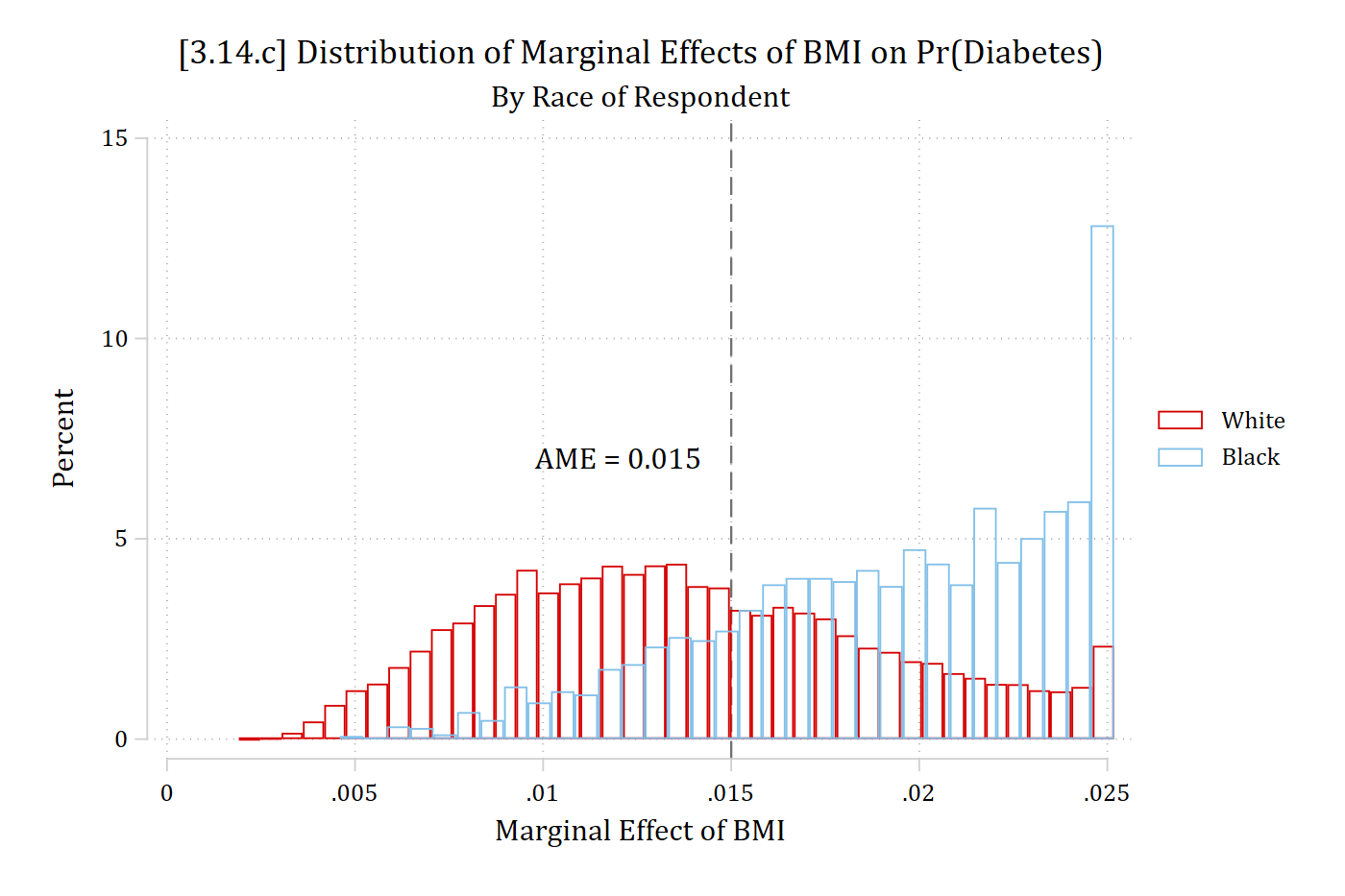
* AMEs for BMI, separate by race of R
twoway (hist MEs_bmi if race == 1, percent fcolor(none) bcolor(red*1.2)) ///
    (hist MEs_bmi if race == 2, percent fcolor(none) bcolor(eltblue)), ///
    xline(.015, lpat(dash)) text(7 .012 "AME = 0.015") xtitle("Marginal Effect
 of BMI") ///
    title("[3.14.c] Distribution of Marginal Effects of BMI on Pr(Diabetes)") 
///
    subtitle("By Race of Respondent") legend(order(1 "White" 2 "Black"))

R

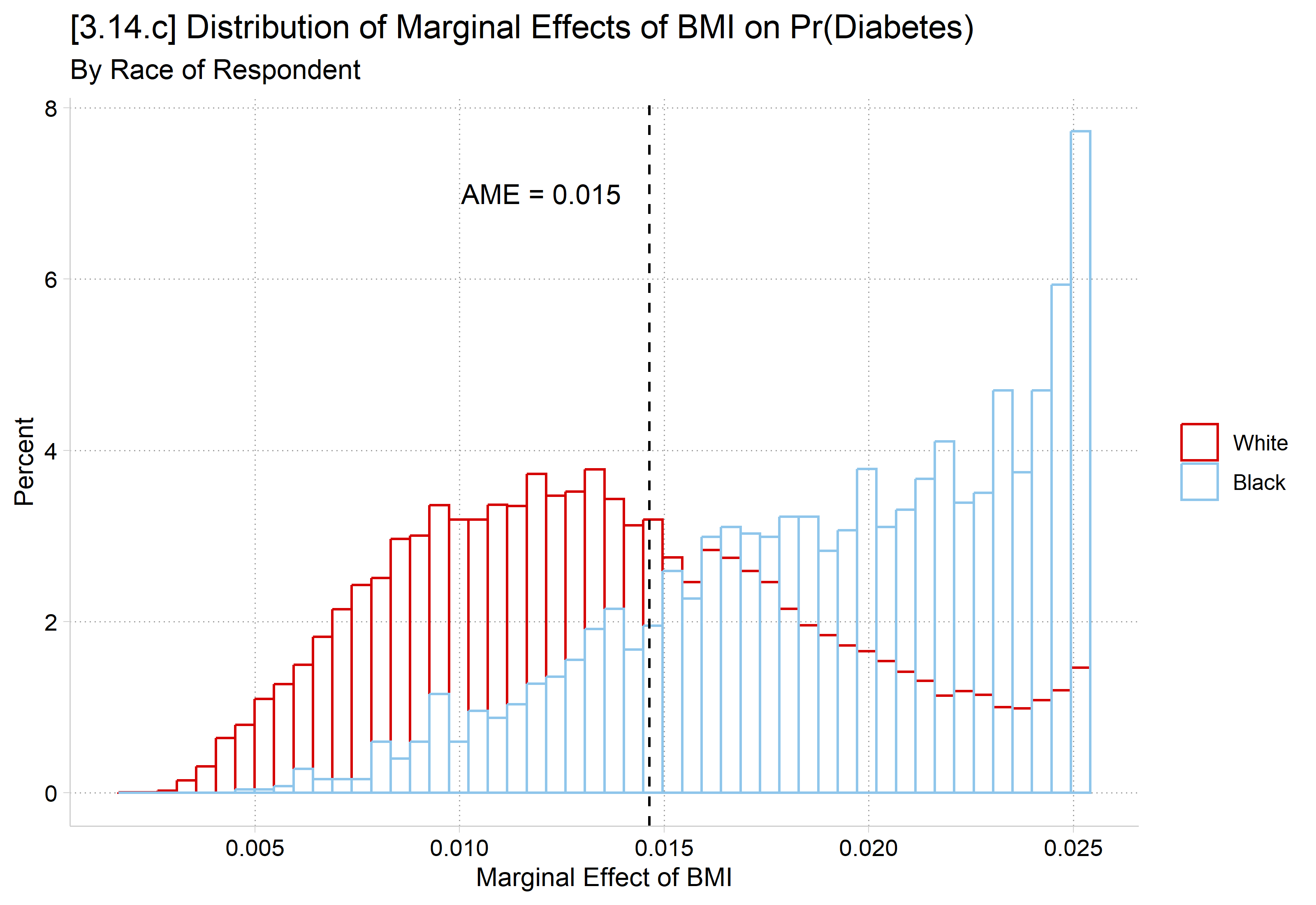
# AMEs for BMI, separate by race of R
ggplot(MEs_bmi, aes(x = estimate, color = black)) +
  geom_histogram(aes(y = after_stat(100 * count / tapply(count, group, sum)[group])),
    bins = 50, fill = NA, position = "identity") +
  geom_vline(xintercept = mean(MEs_bmi$estimate), linetype = "dashed") +
  annotate("text", x = .012, y = 7, label = "AME = 0.015") +
  labs(title = "[3.14.c] Distribution of Marginal Effects of BMI on Pr(Diabetes)",
    subtitle = "By Race of Respondent",
    x = "Marginal Effect of BMI", y = "Percent", color = NULL)

Stata

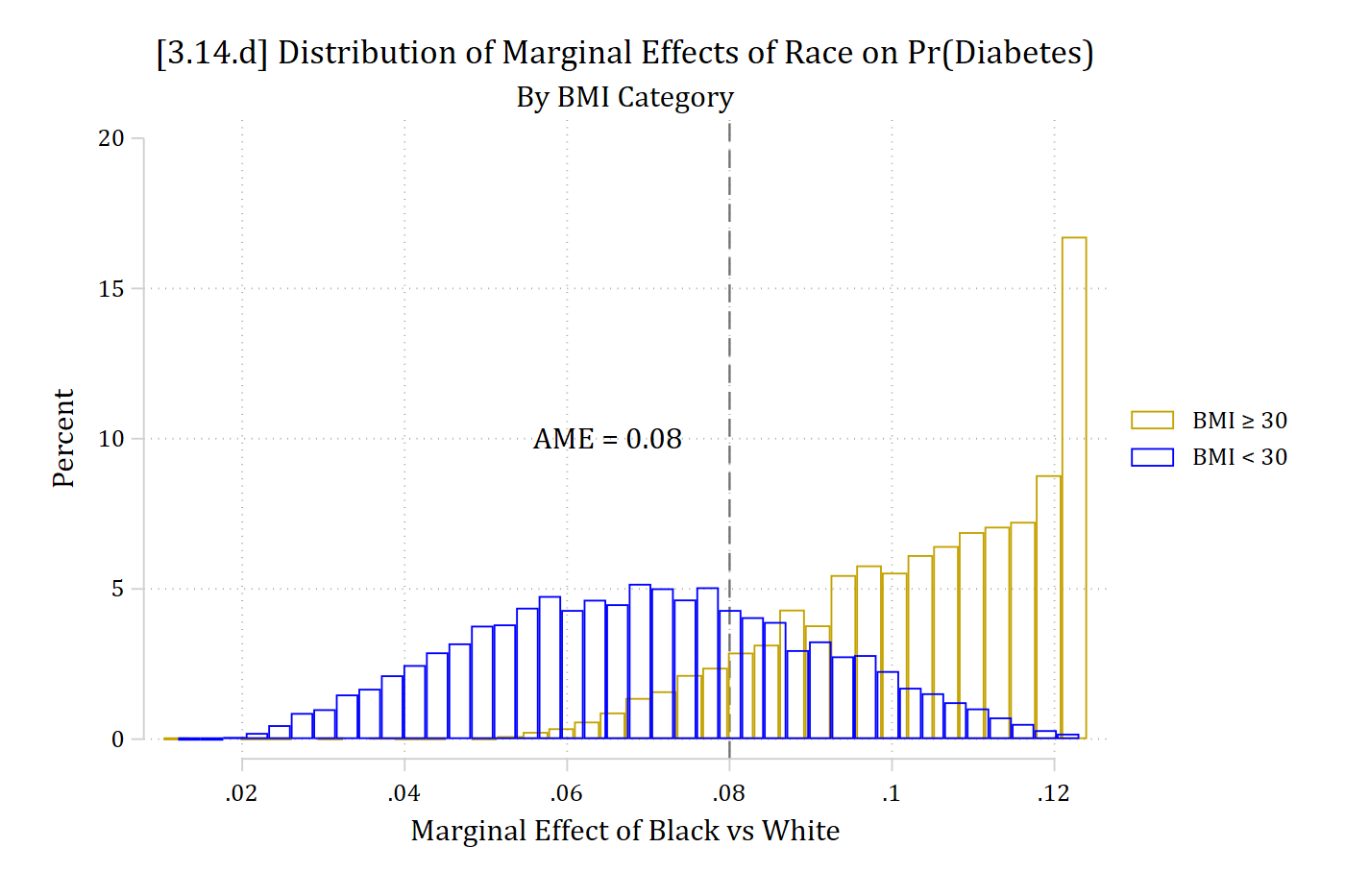
* AMEs for race, separate by BMI group
twoway (hist MEs_black2 if bmi >= 30, percent fcolor(none) bcolor(gold*1.3)) /
//
    (hist MEs_black2 if bmi < 30, percent fcolor(none) bcolor(blue)), ///
    xline(.08, lpat(dash)) text(10 .065 "AME = 0.08") ///
    xtitle("Marginal Effect of Black vs White") ///
    title("[3.14.d] Distribution of Marginal Effects of Race on Pr(Diabetes)")
 ///
    subtitle("By BMI Category") legend(order(1 "BMI {&ge} 30" 2 "BMI {&lt} 30"
))

R

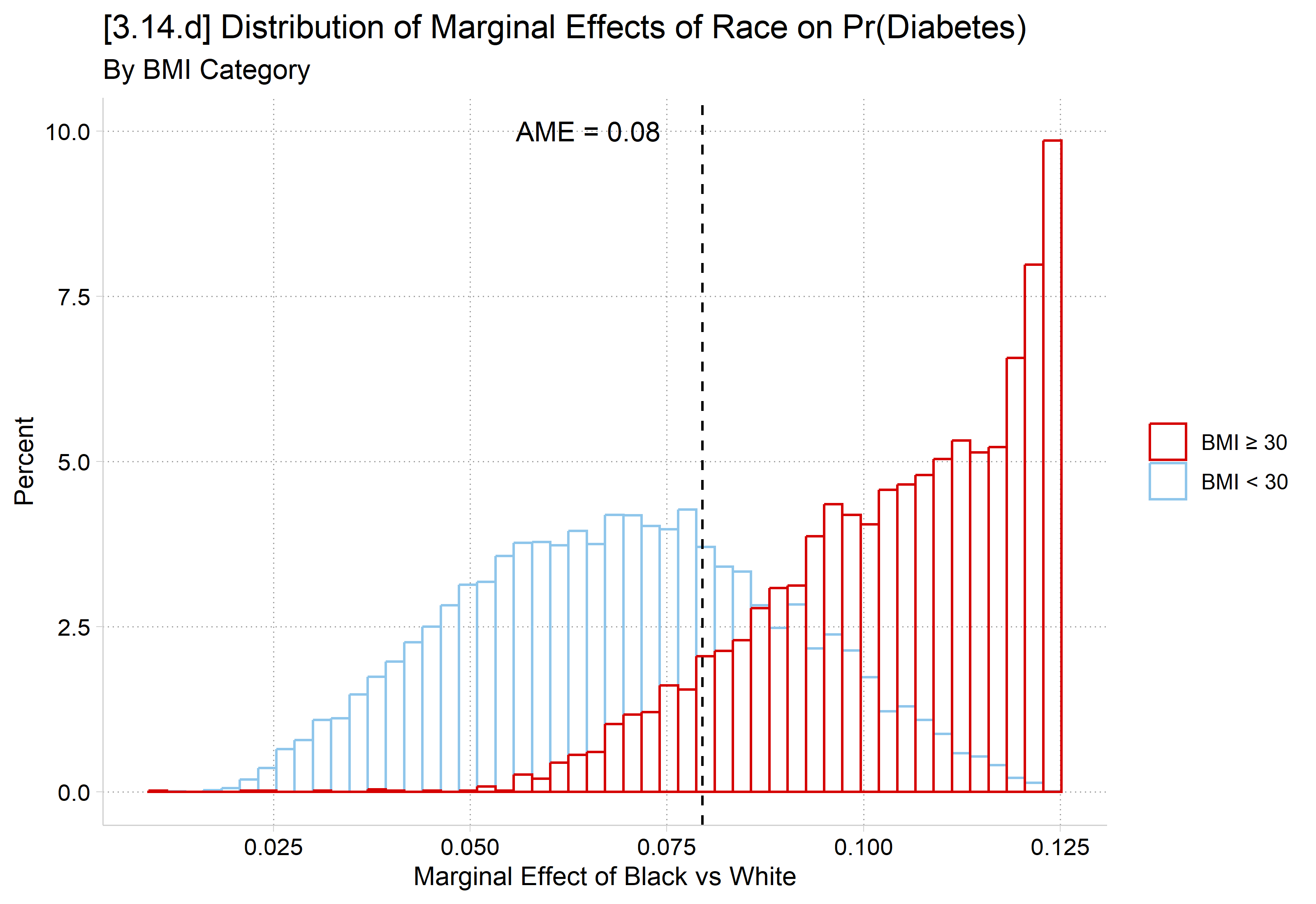
# AMEs for race, separate by BMI group
MEs_black <- MEs_black |> mutate(bmigroup = if_else(bmi >= 30, "BMI ≥ 30", "BMI < 30"))

ggplot(MEs_black, aes(x = estimate, color = bmigroup)) +
  geom_histogram(aes(y = after_stat(100 * count / tapply(count, group, sum)[group])),
    bins = 50, fill = NA, position = "identity") +
  geom_vline(xintercept = mean(MEs_black$estimate), linetype = "dashed") +
  annotate("text", x = .065, y = 10, label = "AME = 0.08") +
  scale_color_discrete(limits = c("BMI ≥ 30", "BMI < 30")) +
  labs(title = "[3.14.d] Distribution of Marginal Effects of Race on Pr(Diabetes)",
    subtitle = "By BMI Category",
    x = "Marginal Effect of Black vs White", y = "Percent", color = NULL)