6.7 Another Negative Binomial Example

use "https://tdmize.github.io/data/data/cda_ah4", clear
(cda_ah4.dta | Add Health Wave 4 - | )
*DV has non-integer values, so need to round to make it work for a count model
replace depressSS = depressSS * 10
(4,812 real changes made)
replace depressSS = round(depressSS, 1)
(3,206 real changes made)
tabstat depressSS, stat(mean var sd) format(%4.2f)
    Variable |      Mean  Variance        SD
-------------+------------------------------
   depressSS |      6.09     21.99      4.69
--------------------------------------------
library(haven)           # import Stata data and labels
library(dplyr)           # data manipulation
library(sjmisc)          # frq() frequency tables
library(tidyr)           # reshape data: pivot_longer()
library(ggplot2)         # graphs
library(MASS)            # negative binomial: glm.nb()
library(pscl)            # odTest()
library(marginaleffects) # predictions and marginal effects
library(cleanplots)      # graph scheme
cleanplots_defaults()

source("https://raw.githubusercontent.com/tdmize/Rfunctions/main/ME_helper_functions.R")

ah4 <- read_dta("https://tdmize.github.io/data/data/cda_ah4.dta")

# DV has non-integer values, so need to round to make it work for a count model
ah4 <- ah4 |> mutate(depressSS = round(depressSS * 10))

ah4 |> summarise(mean = mean(depressSS, na.rm = TRUE), var = var(depressSS, na.rm = TRUE),
  sd = sd(depressSS, na.rm = TRUE))
# A tibble: 1 × 3
   mean   var    sd
  <dbl> <dbl> <dbl>
1  6.09  22.0  4.69
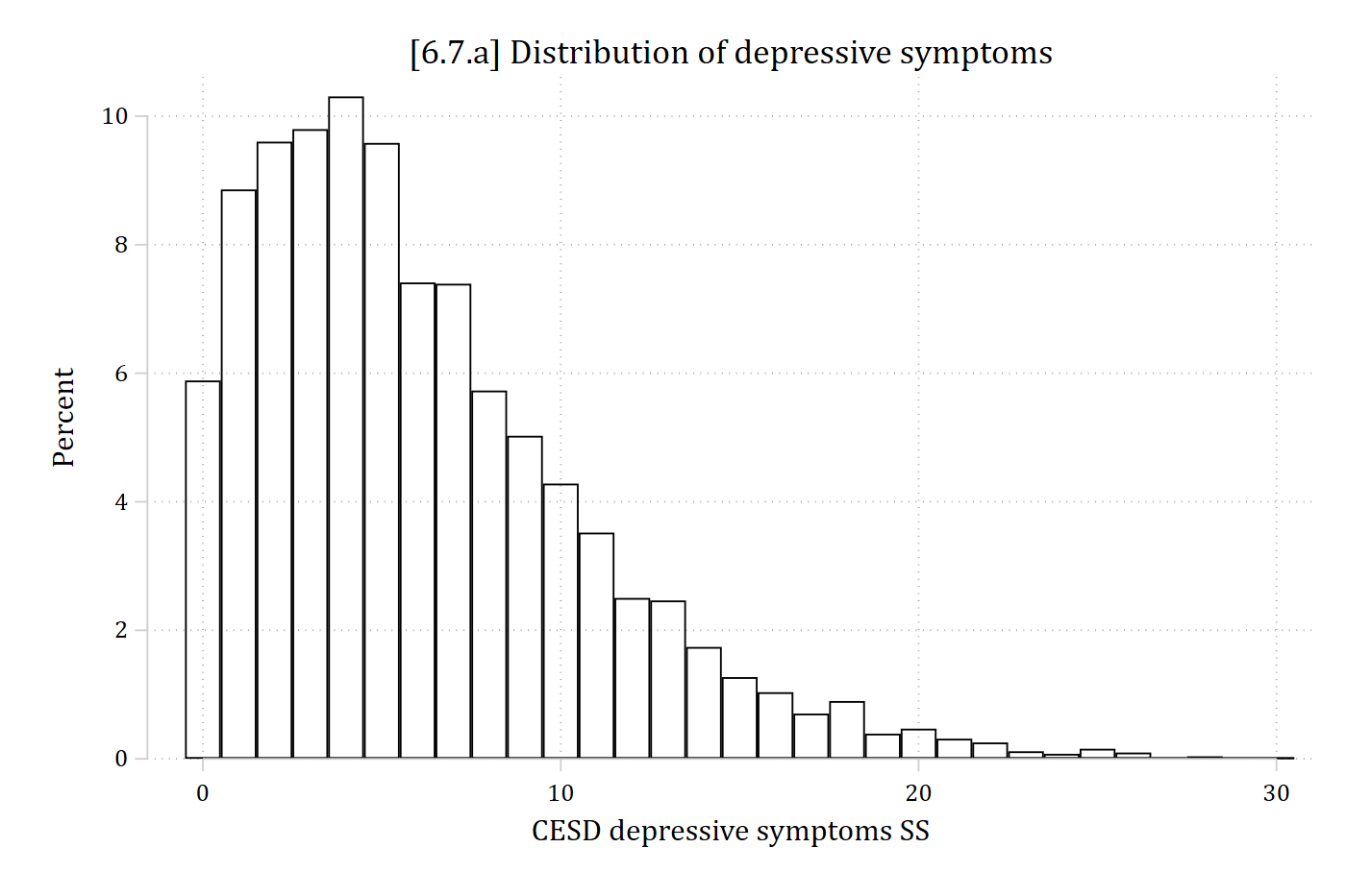
*6.7.a
hist depressSS, percent discrete fcol(none) ///
    title("[6.7.a] Distribution of depressive symptoms")
(start=0, width=1)

[6.7.a] Histogram of the number of depressive symptoms from 0 to 30: most respondents have 1 to 8 symptoms, the peak is about 10% at 4 symptoms, and the distribution has a long right tail.

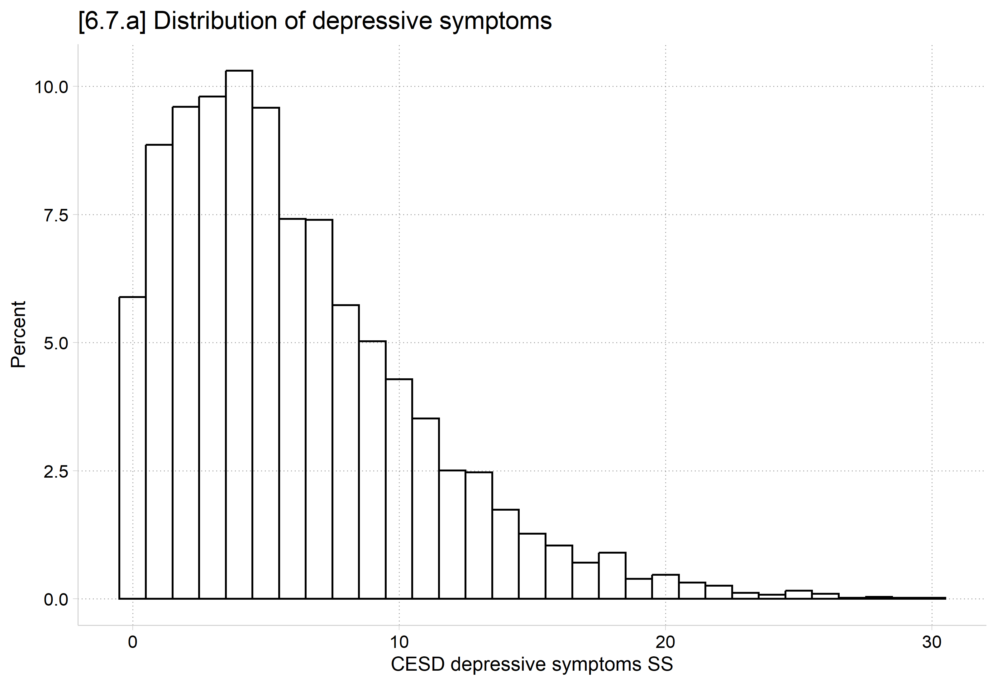
# 6.7.a
ggplot(ah4, aes(x = depressSS)) +
  geom_histogram(aes(y = after_stat(100 * count / sum(count))), binwidth = 1,
    fill = NA, color = "black") +
  labs(title = "[6.7.a] Distribution of depressive symptoms",
    x = "CESD depressive symptoms SS", y = "Percent")

[6.7.a] Histogram of the number of depressive symptoms from 0 to 30: most respondents have 1 to 8 symptoms, the peak is about 10% at 4 symptoms, and the distribution has a long right tail.

*6.7.b - compare predictions to choose model
qui nbreg depressSS i.woman c.role##c.role c.income c.age i.race, irr
qui mgen, pr(0/30) meanpred stub(nb) replace
qui poisson depressSS i.woman c.role##c.role c.income c.age i.race, irr
qui mgen, pr(0/30) meanpred stub(p) replace
twoway connected pobeq ppreq nbpreq pval, ylab(0(.05).2, format(%4.2f)) ///
    xlab(0(5)30) ytitle("Pr(y = k)") xtitle("Number of Depressive Symptoms") /
//
    title("[6.7.b] Comparison of Mean Predictions from Poisson and Negative Bi
nomial") ///
    text(.15 20 "{&mu} = 6.09" " " "{&sigma}{sup:2} = 21.99") ///
    legend(order(1 "Observed" 2 "Poisson" 3 "Neg. Binomial"))

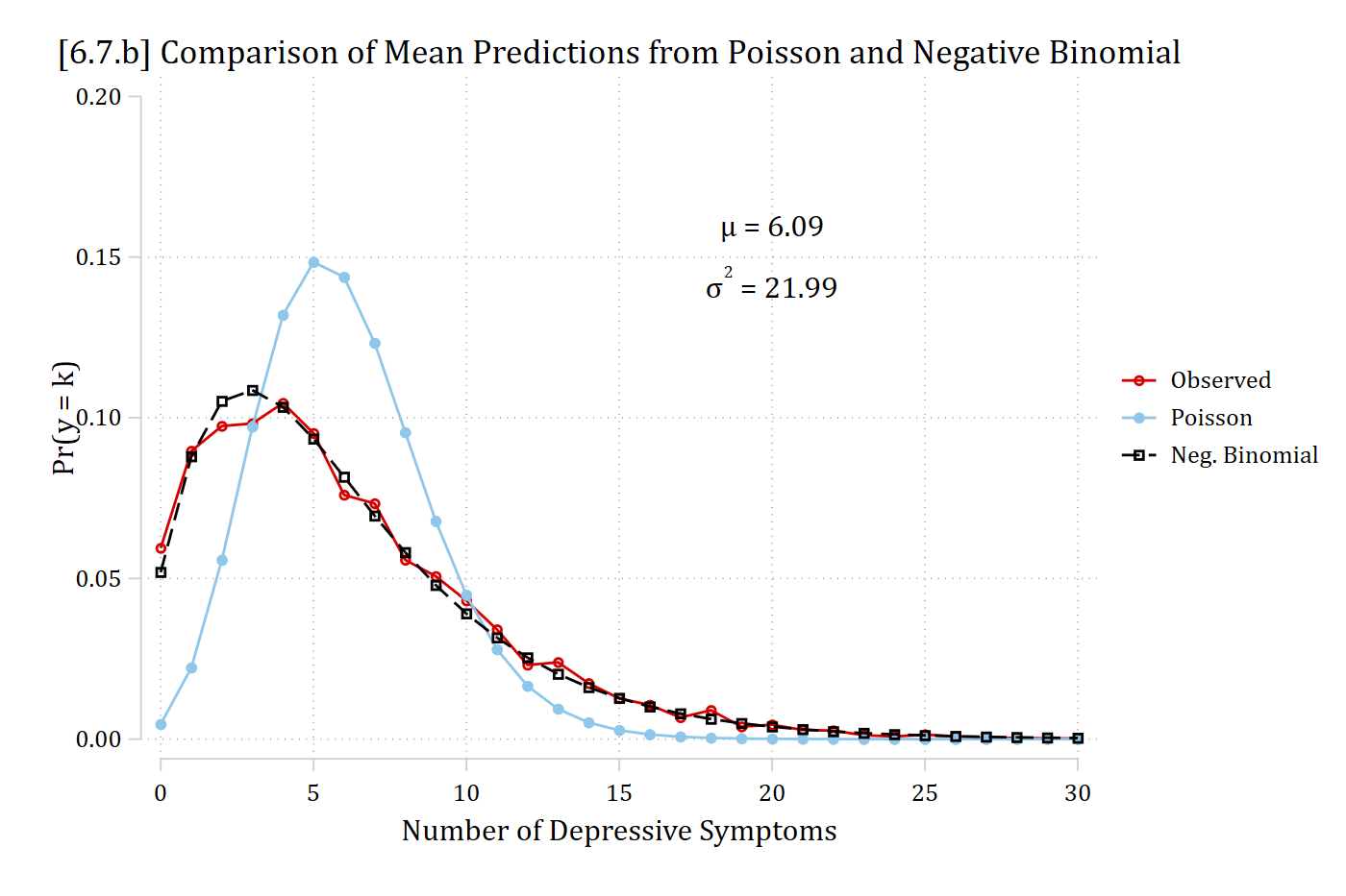
[6.7.b] Observed proportions of each number of depressive symptoms with average predicted probabilities from the Poisson and negative binomial models: the Poisson predictions are too peaked, about 0.15 at 5 symptoms and near 0 at 0 to 1, while the negative binomial predictions closely match the observed proportions across the whole range.

# Keep model variables; drop any missing data
dep <- ah4[c("depressSS", "woman", "role", "income", "age", "race")]
dep <- dep[complete.cases(dep), ]
dep <- dep |> mutate(across(c(woman, race), as_factor))

# 6.7.b - compare predictions to choose model
nbdep <- glm.nb(depressSS ~ woman + poly(role, 2, raw = TRUE) + income + age + race,
  data = dep)
pdep <- glm(depressSS ~ woman + poly(role, 2, raw = TRUE) + income + age + race,
  family = "poisson", data = dep)

meanpred <- data.frame(k = 0:30) |>
  mutate(Observed = sapply(k, function(j) mean(dep$depressSS == j)),
    Poisson = sapply(k, function(j) mean(dpois(j, fitted(pdep)))),
    "Neg. Binomial" = sapply(k, function(j)
      mean(dnbinom(j, size = nbdep$theta, mu = fitted(nbdep))))) |>
  pivot_longer(-k, names_to = "type", values_to = "pr") |>
  mutate(type = factor(type, levels = c("Observed", "Poisson", "Neg. Binomial")))

ggplot(meanpred, aes(x = k, y = pr, color = type)) +
  geom_line() + geom_point() +
  annotate("text", x = 20, y = .15, label = 'mu == "6.09"', parse = TRUE) +
  annotate("text", x = 20, y = .135, label = 'sigma^2 == "21.99"', parse = TRUE) +
  scale_x_continuous(breaks = seq(0, 30, 5)) +
  scale_y_continuous(breaks = seq(0, .2, .05), limits = c(0, .2)) +
  labs(title = "[6.7.b] Comparison of Mean Predictions from Poisson and Negative Binomial",
    x = "Number of Depressive Symptoms", y = "Pr(y = k)", color = NULL)
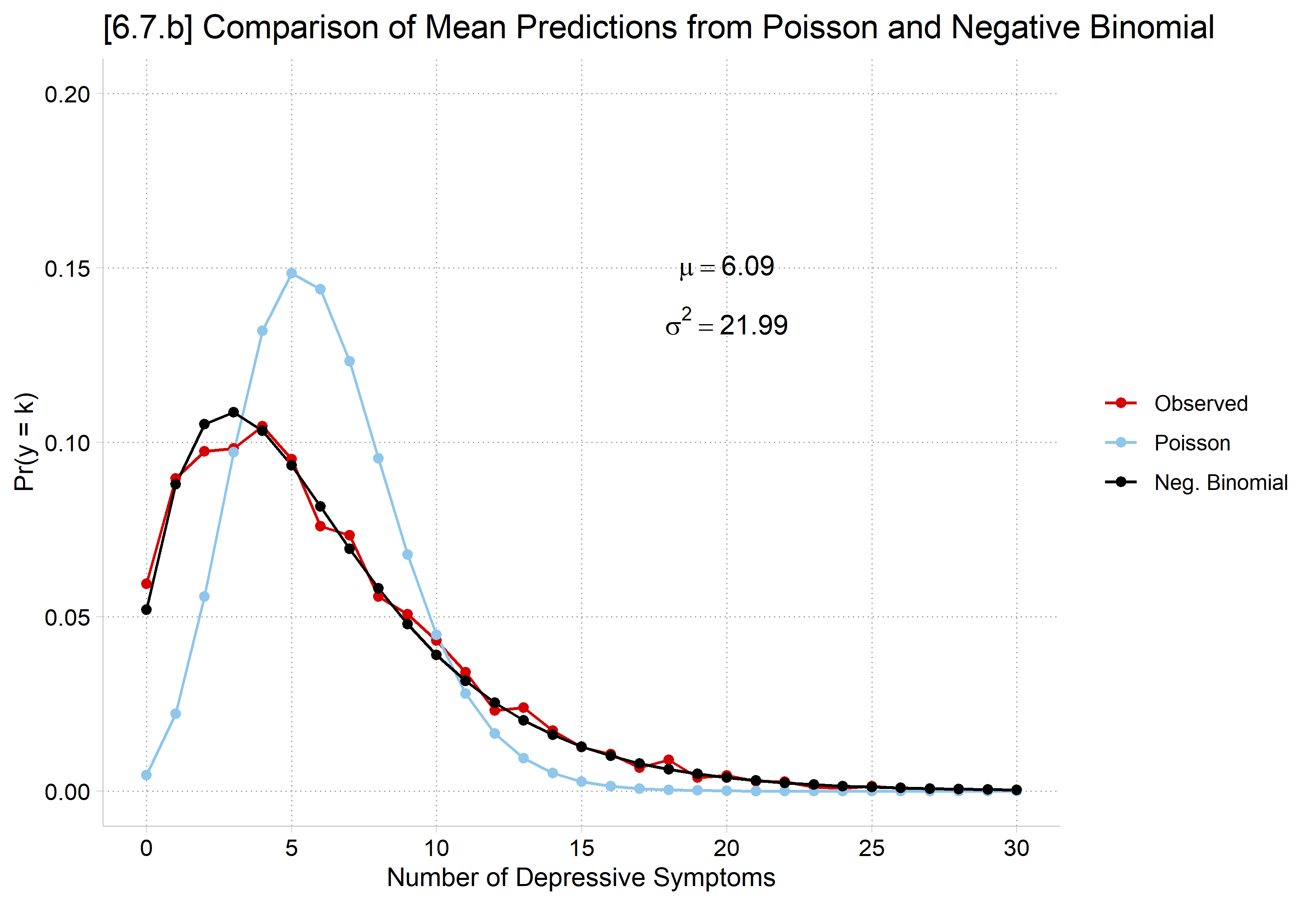
[6.7.b] Observed proportions of each number of depressive symptoms with average predicted probabilities from the Poisson and negative binomial models: the Poisson predictions are too peaked, about 0.15 at 5 symptoms and near 0 at 0 to 1, while the negative binomial predictions closely match the observed proportions across the whole range.

Poisson does quite a bad job; negative binomial is remarkably effective here at matching the true distribution of the DV

nbreg depressSS i.woman c.role##c.role c.income c.age i.race, irr
Fitting Poisson model:

Iteration 0:  Log likelihood = -16083.744  
Iteration 1:  Log likelihood = -16083.732  
Iteration 2:  Log likelihood = -16083.732  

Fitting constant-only model:

Iteration 0:  Log likelihood = -14080.722  
Iteration 1:  Log likelihood =  -13685.13  
Iteration 2:  Log likelihood = -13685.002  
Iteration 3:  Log likelihood = -13685.002  

Fitting full model:

Iteration 0:  Log likelihood = -13519.543  
Iteration 1:  Log likelihood = -13510.817  
Iteration 2:  Log likelihood =   -13510.8  
Iteration 3:  Log likelihood =   -13510.8  

Negative binomial regression                            Number of obs =  4,896
                                                        LR chi2(8)    = 348.41
Dispersion: mean                                        Prob > chi2   = 0.0000
Log likelihood = -13510.8                               Pseudo R2     = 0.0127

-------------------------------------------------------------------------------
    depressSS |        IRR   Std. err.      z    P>|z|     [95% conf. interval]
--------------+----------------------------------------------------------------
        woman |
       Woman  |      1.160      0.026    6.527   0.000        1.110       1.213
         role |      0.832      0.030   -5.031   0.000        0.775       0.894
              |
c.role#c.role |      1.010      0.003    2.979   0.003        1.003       1.016
              |
       income |      0.996      0.000   -9.581   0.000        0.995       0.997
          age |      1.011      0.006    1.798   0.072        0.999       1.023
              |
         race |
       Black  |      1.109      0.029    4.029   0.000        1.055       1.167
Native Ame..  |      0.974      0.123   -0.213   0.832        0.760       1.247
       Asian  |      1.180      0.074    2.639   0.008        1.043       1.334
              |
        _cons |      9.139      1.806   11.196   0.000        6.204      13.462
--------------+----------------------------------------------------------------
     /lnalpha |     -0.898      0.030                        -0.957      -0.839
--------------+----------------------------------------------------------------
        alpha |      0.407      0.012                         0.384       0.432
-------------------------------------------------------------------------------
Note: Estimates are transformed only in the first equation to incidence-rate
      ratios.
Note: _cons estimates baseline incidence rate.
LR test of alpha=0: chibar2(01) = 5145.87              Prob >= chibar2 = 0.000
est store nbmod
summary(nbdep)

Call:
glm.nb(formula = depressSS ~ woman + poly(role, 2, raw = TRUE) + 
    income + age + race, data = dep, init.theta = 2.454375796, 
    link = log)

Coefficients:
                             Estimate Std. Error z value Pr(>|z|)    
(Intercept)                 2.2125638  0.1985011  11.146  < 2e-16 ***
womanWoman                  0.1487557  0.0227688   6.533 6.43e-11 ***
poly(role, 2, raw = TRUE)1 -0.1834645  0.0366831  -5.001 5.69e-07 ***
poly(role, 2, raw = TRUE)2  0.0096333  0.0032552   2.959  0.00308 ** 
income                     -0.0041731  0.0004426  -9.429  < 2e-16 ***
age                         0.0108292  0.0060470   1.791  0.07332 .  
raceBlack                   0.1036533  0.0257178   4.030 5.57e-05 ***
raceNative American        -0.0268315  0.1257104  -0.213  0.83098    
raceAsian                   0.1651477  0.0625115   2.642  0.00824 ** 
---
Signif. codes:  0 '***' 0.001 '**' 0.01 '*' 0.05 '.' 0.1 ' ' 1

(Dispersion parameter for Negative Binomial(2.4544) family taken to be 1)

    Null deviance: 5834.3  on 4895  degrees of freedom
Residual deviance: 5471.6  on 4887  degrees of freedom
AIC: 27042

Number of Fisher Scoring iterations: 1

              Theta:  2.4544 
          Std. Err.:  0.0739 

 2 x log-likelihood:  -27021.5990 
# Exponentiated coefficients
exp(coef(nbdep))
               (Intercept)                 womanWoman poly(role, 2, raw = TRUE)1 
                 9.1391170                  1.1603895                  0.8323814 
poly(role, 2, raw = TRUE)2                     income                        age 
                 1.0096798                  0.9958356                  1.0108881 
                 raceBlack        raceNative American                  raceAsian 
                 1.1092158                  0.9735253                  1.1795674 
odTest(nbdep)
Likelihood ratio test of H0: Poisson, as restricted NB model:
n.b., the distribution of the test-statistic under H0 is non-standard
e.g., see help(odTest) for details/references

Critical value of test statistic at the alpha= 0.05 level: 2.7055 
Chi-Square Test Statistic =  5145.8655 p-value = < 2.2e-16 
*6.7.c - Predictions on rate/count
est restore nbmod
(results nbmod are active now)
qui margins woman, at(role=(0(1)10))
marginsplot, recastci(rline) ciopts(lpat(dash) col(gs12)) ylab(0(5)17) ///
    ytitle("# of Depressive Symptoms") ///
    title("[6.7.c] Predicted Number of Depressive Symptoms by Social Roles Hel
d and Gender", size(medium))
Variables that uniquely identify margins: role woman

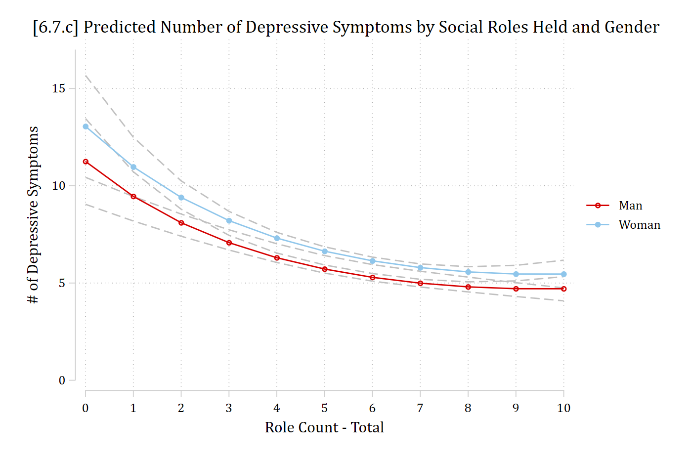
[6.7.c] Predicted number of depressive symptoms by number of social roles held, with confidence intervals: predictions fall steeply from about 11 (men) and 13 (women) with no roles to about 6 with 5 roles, then level off near 5 with 10 roles; women are predicted to have slightly more symptoms than men throughout.

# 6.7.c - Predictions on rate/count
plot_predictions(nbdep, by = c("role", "woman"),
  newdata = datagrid(role = 0:10, woman = unique, grid_type = "counterfactual")) +
  scale_x_continuous(breaks = 0:10) +
  scale_y_continuous(breaks = seq(0, 15, 5)) +
  coord_cartesian(ylim = c(0, 17)) +
  labs(title = "[6.7.c] Predicted Number of Depressive Symptoms by Social Roles Held and Gender",
    x = "Role Count - Total", y = "# of Depressive Symptoms", color = NULL, fill = NULL)

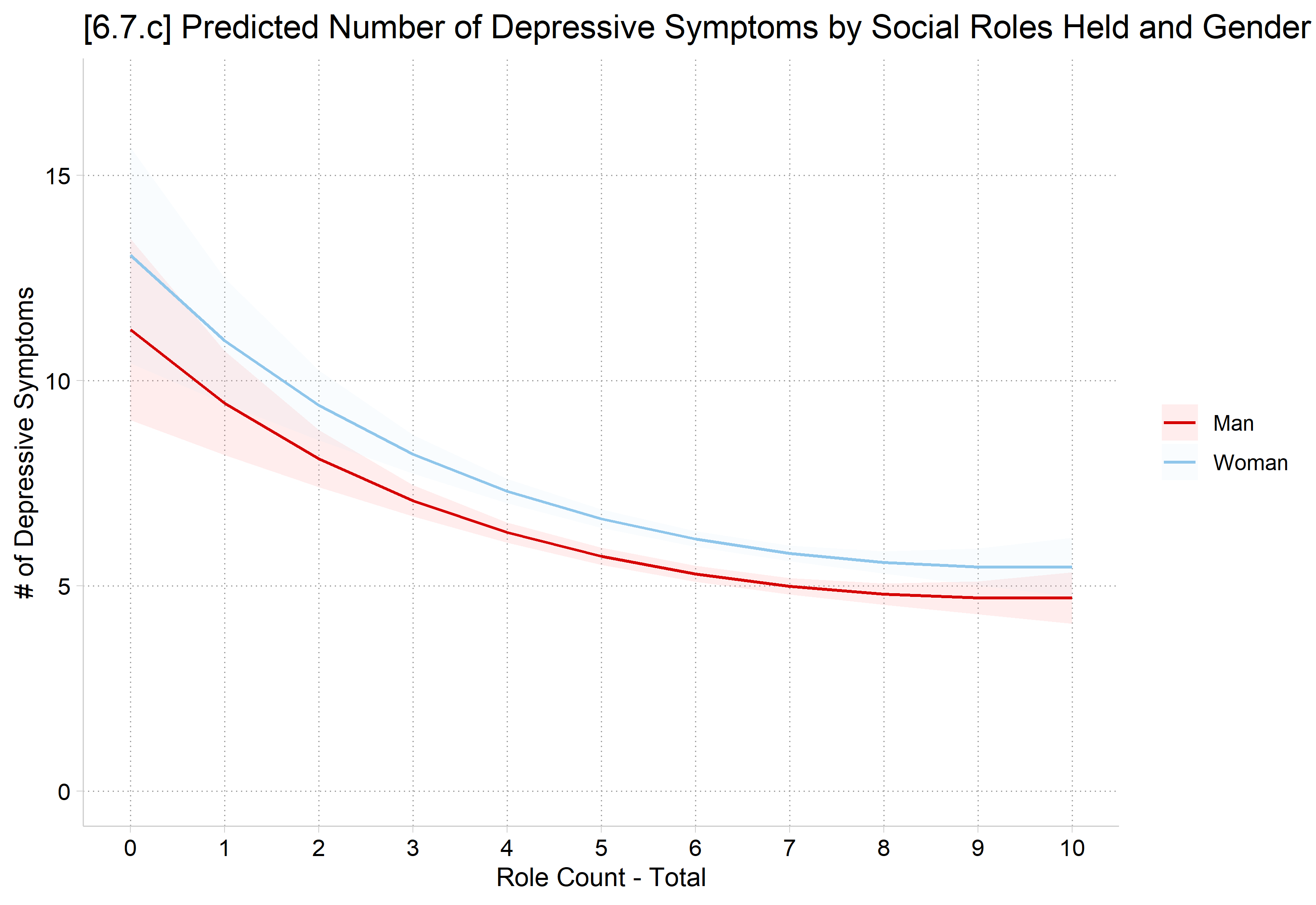
[6.7.c] Predicted number of depressive symptoms by number of social roles held, with confidence intervals: predictions fall steeply from about 11 (men) and 13 (women) with no roles to about 6 with 5 roles, then level off near 5 with 10 roles; women are predicted to have slightly more symptoms than men throughout.

AMEs on the rate of depressive symptoms

*MEs on the rate
mecompare woman role, model(nbmod)
Predicting: Predicted number of events
Marginal effects (N_nbmod=4896)

                                 |  ME #   Estimate         SE      P>|z|
---------------------------------+---------------------------------------
woman                            |                                       
                 Woman - Man     |                                       
                           nbmod |     1      0.889      0.136      0.000
---------------------------------+---------------------------------------
role + 1 (centered)              |                                       
                           nbmod |     2     -0.458      0.047      0.000
# Center changes in continuous IVs on each observation's value (as mecompare does)
options(marginaleffects_contrast_direction = "center")

# MEs on the rate
avg_comparisons(nbdep, variables = list(woman = "reference", role = 1))

  Term    Contrast Estimate Std. Error     z Pr(>|z|)    S  2.5 % 97.5 %
 role  +1            -0.458     0.0471 -9.73   <0.001 72.0 -0.550 -0.366
 woman Woman - Man    0.889     0.1356  6.56   <0.001 34.1  0.624  1.155

Type: response

On average, women report about 0.89 more depressive symptoms than men

On average, an additional role is predicted to reduce depressive symptoms by 0.46

  • Because of the pronounced nonlinearities, do not want to only report average effect for roles (see the graph above)
    • Based on graph (and/or percentiles), show effects at low value, and high value
mecompare role, model(nbmod) start(role=(0 7)) uncenter
Predicting: Predicted number of events
Marginal effects (N_nbmod=4896)

                                 |  ME #   Estimate         SE      P>|z|
---------------------------------+---------------------------------------
role + 1 (uncentered)            |                                       
                            at 0 |     1     -1.955      0.536      0.000
                            at 7 |     2     -0.208      0.076      0.006
# Forward (uncentered) changes from the values given in datagrid()
options(marginaleffects_contrast_direction = "forward")

avg_comparisons(nbdep, variables = list(role = 1), by = "role",
  newdata = datagrid(role = c(0, 7), grid_type = "counterfactual"))

 role Estimate Std. Error     z Pr(>|z|)    S  2.5 %  97.5 %
    0   -1.955     0.5393 -3.62  < 0.001 11.8 -3.012 -0.8978
    7   -0.208     0.0767 -2.71  0.00675  7.2 -0.358 -0.0575

Term: role
Type: response
Comparison: +1

The average effect of an additional social role is a 0.46 reduction in depressive symptoms. However, social roles have a diminishing effect. For example, for someone with zero social roles, gaining an additional role is predicted to reduce depressive symptoms by almost 2. In contrast, a change from 7 to 8 social roles is predicted to reduce depressive symptoms by only about 0.21.

Bonus: difference in marginal effects

  • In Stata, test the difference in the two MEs above with metest
  • In R, specify a difference in MEs as a hypothesis on avg_comparisons
metest 2 - 1
                                 |  estimate         se     pvalue 
---------------------------------+--------------------------------
             role_at7 - role_at0 |     1.747      0.592      0.003 
avg_comparisons(nbdep, variables = list(role = 1), by = "role",
  newdata = datagrid(role = c(0, 7), grid_type = "counterfactual"),
  hypothesis = "b2 - b1 = 0")

 Hypothesis Estimate Std. Error    z Pr(>|z|)   S 2.5 % 97.5 %
    b2-b1=0     1.75      0.596 2.93  0.00336 8.2  0.58   2.91

Type: response

The marginal effect of a +1 increase in social roles is larger (more negative) at 0 roles than at 7 roles (difference p < .01).

Effects on cumulative probabilities

  • Scores above 12 on the CES-D depression scale are considered “at risk” for depression (e.g., see Roberts et al. 1990; McLeod et al. 2012)
  • Rather than dichotomizing the depression scale for analysis you can treat this properly as a count and analyze cumulative probabilities for 12 or more symptoms
    • Or for 11 or fewer symptoms (i.e., “not at risk”)
*6.7.d - Predictions for low range of depressive symptoms (0 to 11)
est restore nbmod
(results nbmod are active now)
qui margins woman, at(role=(0(1)10)) predict(pr(0,11))
marginsplot, recastci(rline) ciopts(lpat(dash) col(gs12)) ylab(.2(.2)1) ///
    ytitle("Pr(Not at Risk of Depression)") ///
    title("[6.7.d] Probability of Having 11 or Fewer Depressive Symptoms (i.e.
 Not At Risk)", size(medium))
Variables that uniquely identify margins: role woman

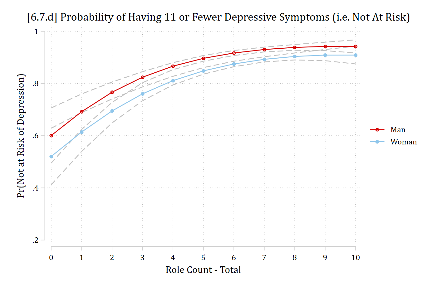
[6.7.d] Probability of having 11 or fewer depressive symptoms (not at risk of depression) by number of social roles, with confidence intervals: it rises from about 0.60 (men) and 0.52 (women) with no roles to about 0.94 and 0.91 with 10 roles.

# 6.7.d - Predictions for low range of depressive symptoms (0 to 11)
pr0_11 <- predictions(nbdep, type = "response",
  newdata = datagrid(role = 0:10, woman = unique, grid_type = "counterfactual"),
  hypothesis = ~ I(mean(pnbinom(11, size = nbdep$theta, mu = x))) | role + woman)

ggplot(pr0_11, aes(role, estimate, ymin = conf.low, ymax = conf.high, color = woman, fill = woman)) +
  geom_ribbon(alpha = .2, color = NA) + geom_line() +
  scale_x_continuous(breaks = 0:10) +
  scale_y_continuous(breaks = seq(.2, 1, .2), limits = c(.2, 1)) +
  labs(title = "[6.7.d] Probability of Having 11 or Fewer Depressive Symptoms (i.e. Not At Risk)",
    x = "Role Count - Total", y = "Pr(Not at Risk of Depression)", color = NULL, fill = NULL)

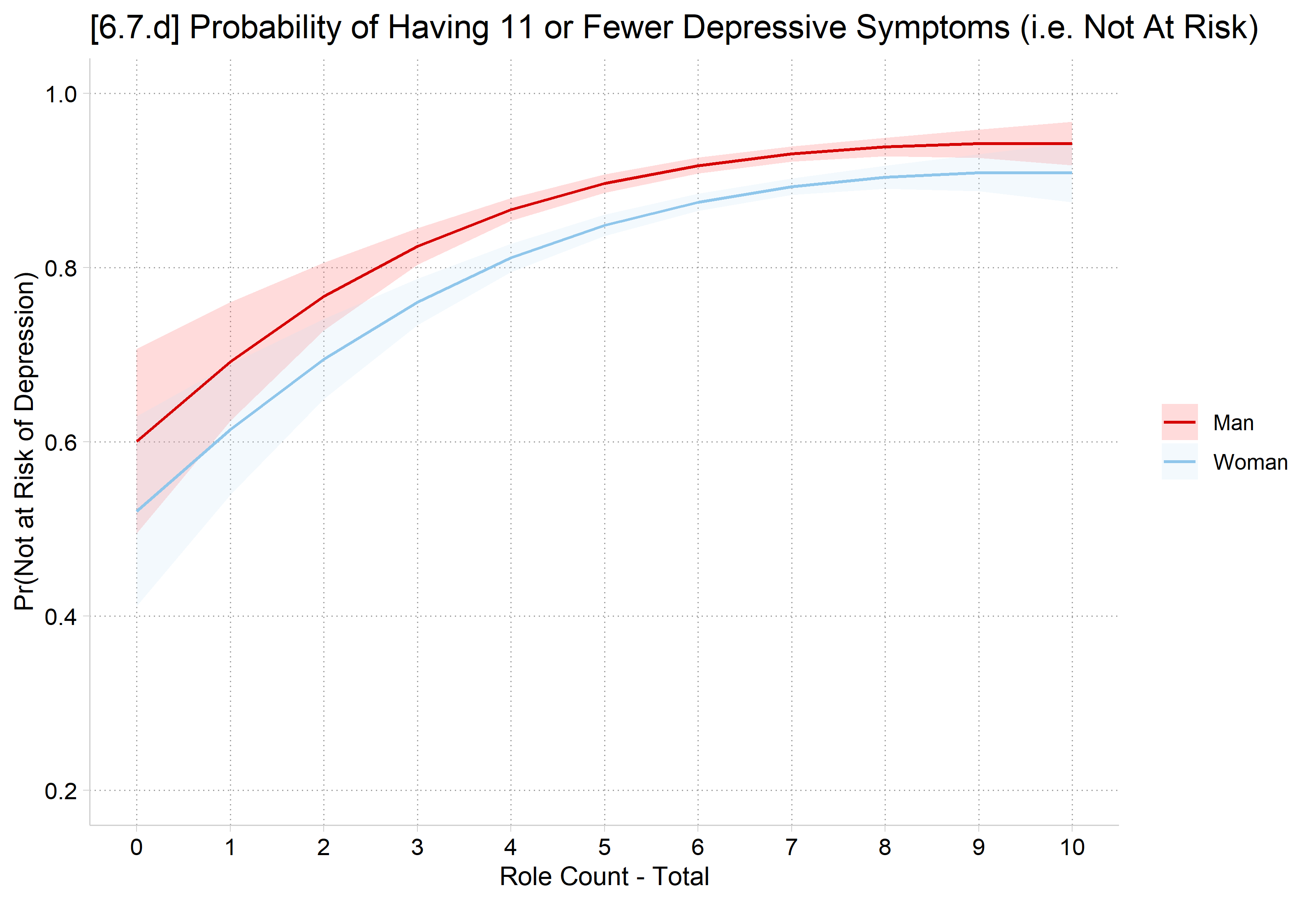
[6.7.d] Probability of having 11 or fewer depressive symptoms (not at risk of depression) by number of social roles, with confidence intervals: it rises from about 0.60 (men) and 0.52 (women) with no roles to about 0.94 and 0.91 with 10 roles.

Nominal IVs

  • Adding two nominal IVs to our model for depressive symptoms
fre educ orient5 if educ < . & orient5 < .
educ -- Education Categories
-----------------------------------------------------------------------------
                                |      Freq.    Percent      Valid       Cum.
--------------------------------+--------------------------------------------
Valid   0 No High School Degree |        385       7.61       7.61       7.61
        1 High School Degree    |        994      19.64      19.64      27.25
        2 Some College          |       2019      39.90      39.90      67.15
        3 College Degree        |       1208      23.87      23.87      91.03
        4 Graduate Degree       |        454       8.97       8.97     100.00
        Total                   |       5060     100.00     100.00           
-----------------------------------------------------------------------------

orient5 -- Sexual Orientation Identity 5
--------------------------------------------------------------------
                       |      Freq.    Percent      Valid       Cum.
-----------------------+--------------------------------------------
Valid   1 Heterosexual |       4363      86.23      86.23      86.23
        2 MostlyHetero |        509      10.06      10.06      96.28
        3 Bisexual     |         86       1.70       1.70      97.98
        4 MostlyGay    |         40       0.79       0.79      98.77
        5 Gay          |         62       1.23       1.23     100.00
        Total          |       5060     100.00     100.00           
--------------------------------------------------------------------
qui nbreg depressSS i.woman i.educ i.orient5 c.age i.race, irr
est store nbnom
# Keep model variables; drop any missing data
nom <- ah4[c("depressSS", "woman", "educ", "orient5", "age", "race")]
nom <- nom[complete.cases(nom), ]
nom <- nom |> mutate(across(c(woman, educ, orient5, race), as_factor))

# Frequencies for those with valid values on both IVs
nomfre <- ah4[!is.na(ah4$educ) & !is.na(ah4$orient5), ]
frq(nomfre$educ)
Education Categories (x) <numeric> 
# total N=5060 valid N=5060 mean=2.07 sd=1.05

Value |                 Label |    N | Raw % | Valid % | Cum. %
---------------------------------------------------------------
    0 | No High School Degree |  385 |  7.61 |    7.61 |   7.61
    1 |    High School Degree |  994 | 19.64 |   19.64 |  27.25
    2 |          Some College | 2019 | 39.90 |   39.90 |  67.15
    3 |        College Degree | 1208 | 23.87 |   23.87 |  91.03
    4 |       Graduate Degree |  454 |  8.97 |    8.97 | 100.00
 <NA> |                  <NA> |    0 |  0.00 |    <NA> |   <NA>
frq(nomfre$orient5)
Sexual Orientation Identity 5 (x) <numeric> 
# total N=5060 valid N=5060 mean=1.21 sd=0.63

Value |        Label |    N | Raw % | Valid % | Cum. %
------------------------------------------------------
    1 | Heterosexual | 4363 | 86.23 |   86.23 |  86.23
    2 | MostlyHetero |  509 | 10.06 |   10.06 |  96.28
    3 |     Bisexual |   86 |  1.70 |    1.70 |  97.98
    4 |    MostlyGay |   40 |  0.79 |    0.79 |  98.77
    5 |          Gay |   62 |  1.23 |    1.23 | 100.00
 <NA> |         <NA> |    0 |  0.00 |    <NA> |   <NA>
nbnom <- glm.nb(depressSS ~ woman + educ + orient5 + age + race, data = nom)
*6.7.e - Plots of predictions
qui margins educ, post
coefplot, vertical recast(bar) barw(0.5) color(eltblue*.7) ///
    ciopts(recast(rcap) color(gs8)) citop xlabel(, alternate) ///
    ylab(0(1)10) ytitle("# of depressive symptoms") ///
    title("Educational attainment") name(pr_educ, replace)
est restore nbnom
(results nbnom are active now)
qui margins orient5, post
coefplot, vertical recast(bar) barw(0.5) color(*.7) ///
    ciopts(recast(rcap) color(gs8)) citop xlabel(, alternate) ///
    ylab(0(1)10) ytitle("# of depressive symptoms") ///
    title("Sexual orientation identity") name(pr_orient, replace)
graph combine pr_educ pr_orient, ///
    title("[6.7.e] Predicted number of depressive symptoms, by education and s
exuality")

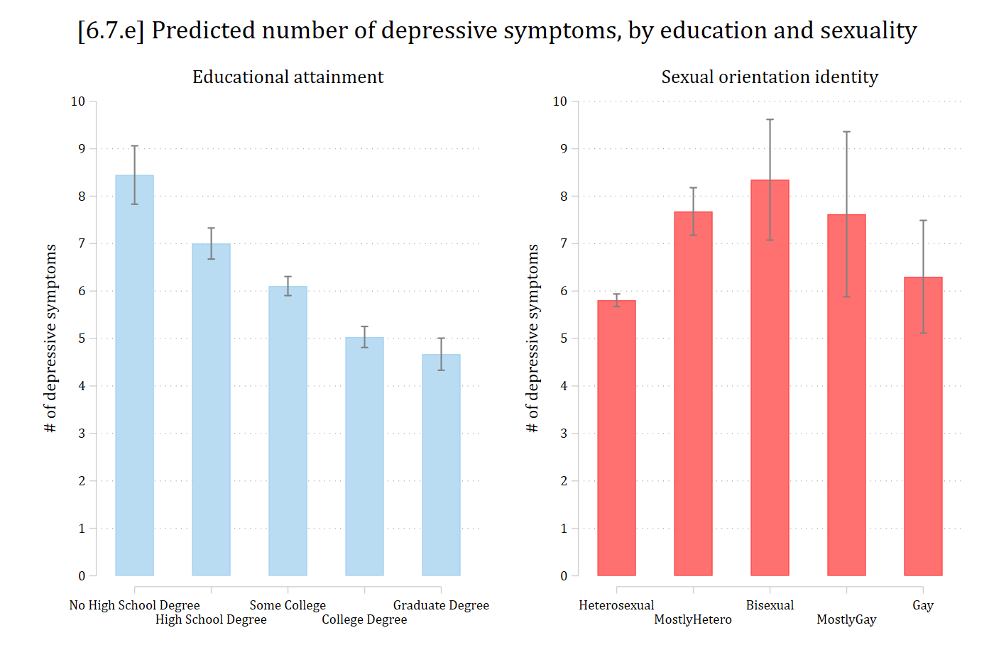
[6.7.e] Two bar charts of the predicted number of depressive symptoms with confidence intervals: by education, from about 8.4 with no high school degree down to about 4.7 with a graduate degree; by sexual orientation identity, about 5.8 for heterosexual, 7.7 for mostly heterosexual, 8.3 for bisexual, 7.6 for mostly gay, and 6.3 for gay respondents.

# 6.7.e - Plots of predictions
pr_educ <- avg_predictions(nbnom, by = "educ",
  newdata = datagrid(educ = unique, grid_type = "counterfactual"))
pr_orient <- avg_predictions(nbnom, by = "orient5",
  newdata = datagrid(orient5 = unique, grid_type = "counterfactual"))

pr_nom <- bind_rows(
  "Educational attainment" = mutate(pr_educ, group = as.character(educ)),
  "Sexual orientation identity" = mutate(pr_orient, group = as.character(orient5)),
  .id = "iv") |>
  mutate(group = factor(group, levels = unique(group)))

ggplot(pr_nom, aes(x = group, y = estimate, fill = iv)) +
  geom_col(width = .5) +
  geom_errorbar(aes(ymin = conf.low, ymax = conf.high), width = .1, color = "gray50") +
  facet_wrap(~ iv, scales = "free_x") +
  scale_x_discrete(labels = scales::label_wrap(12)) +
  scale_y_continuous(breaks = 0:10, limits = c(0, 10)) +
  labs(title = "[6.7.e] Predicted number of depressive symptoms, by education and sexuality",
    x = NULL, y = "# of depressive symptoms") +
  theme(legend.position = "none")

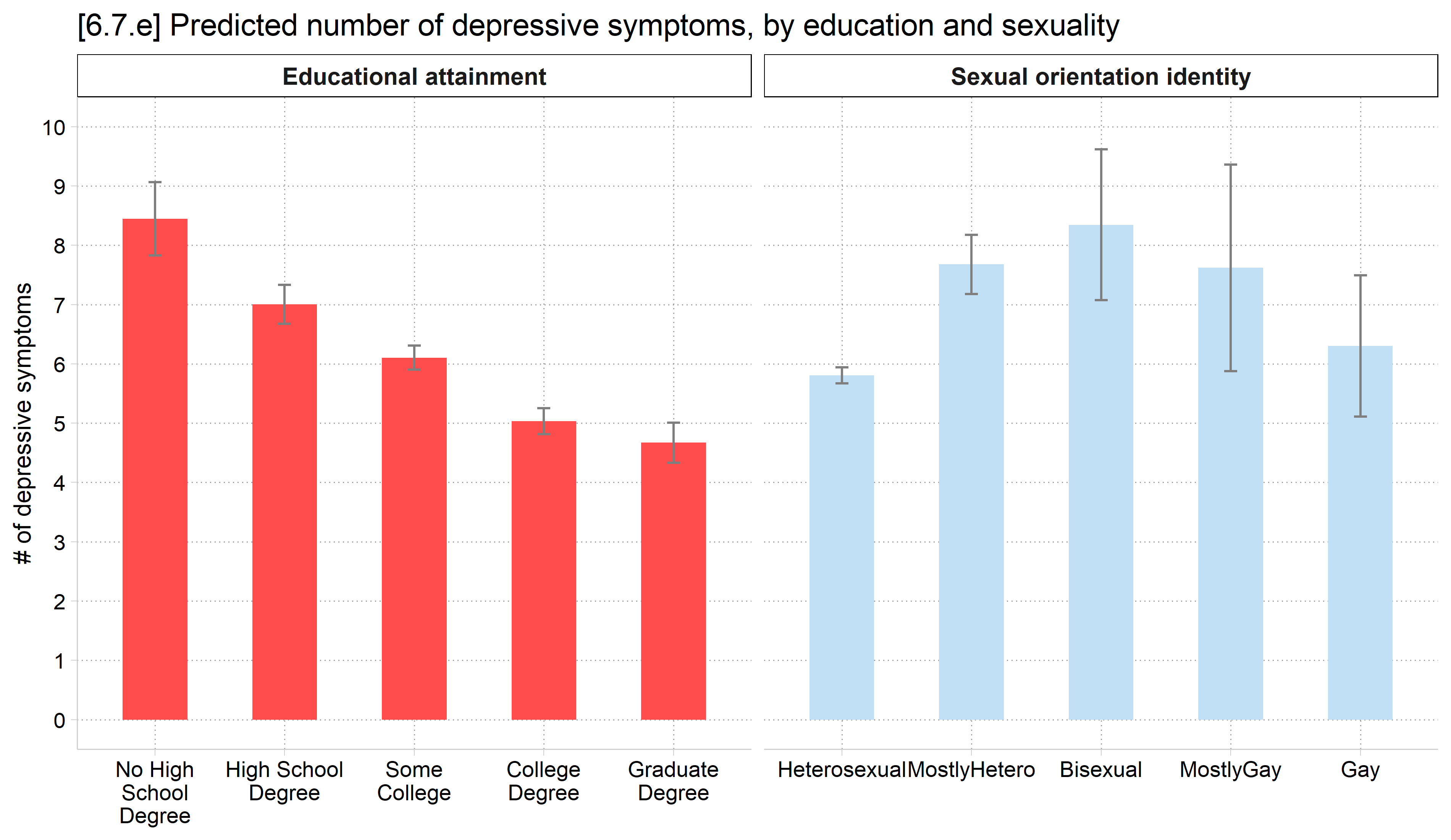
[6.7.e] Two bar charts of the predicted number of depressive symptoms with confidence intervals: by education, from about 8.4 with no high school degree down to about 4.7 with a graduate degree; by sexual orientation identity, about 5.8 for heterosexual, 7.7 for mostly heterosexual, 8.3 for bisexual, 7.6 for mostly gay, and 6.3 for gay respondents.

Marginal effects

  • The default coefficient and marginal effect interpretations will be contrasts with an omitted reference category
    • Ask for all pairwise comparisons with the pwcompare option of mecompare or ask for “pairwise” with avg_comparisons
      • But, be careful with Type I errors (false positives) given so many contrasts tested
*MEs; all pairwise comparisons with pwcompare
mecompare educ orient5, model(nbnom) pwcompare
Predicting: Predicted number of events
Marginal effects (N_nbnom=5056)

                                 |  ME #   Estimate         SE      P>|z|
---------------------------------+---------------------------------------
educ                             |                                       
    High School - No High Sc     |                                       
                           nbnom |     1     -1.444      0.354      0.000
    Some Colleg - No High Sc     |                                       
                           nbnom |     2     -2.341      0.330      0.000
    College Deg - No High Sc     |                                       
                           nbnom |     3     -3.413      0.335      0.000
    Graduate De - No High Sc     |                                       
                           nbnom |     4     -3.776      0.359      0.000
    Some Colleg - High Schoo     |                                       
                           nbnom |     5     -0.897      0.196      0.000
    College Deg - High Schoo     |                                       
                           nbnom |     6     -1.969      0.203      0.000
    Graduate De - High Schoo     |                                       
                           nbnom |     7     -2.333      0.241      0.000
    College Deg - Some Colle     |                                       
                           nbnom |     8     -1.073      0.153      0.000
    Graduate De - Some Colle     |                                       
                           nbnom |     9     -1.436      0.201      0.000
    Graduate De - College De     |                                       
                           nbnom |    10     -0.363      0.207      0.079
---------------------------------+---------------------------------------
orient5                          |                                       
    MostlyHeter - Heterosexu     |                                       
                           nbnom |    11      1.871      0.265      0.000
     Bisexual - Heterosexual     |                                       
                           nbnom |    12      2.540      0.653      0.000
    MostlyGay - Heterosexual     |                                       
                           nbnom |    13      1.814      0.890      0.042
          Gay - Heterosexual     |                                       
                           nbnom |    14      0.496      0.610      0.416
     Bisexual - MostlyHetero     |                                       
                           nbnom |    15      0.669      0.694      0.335
    MostlyGay - MostlyHetero     |                                       
                           nbnom |    16     -0.057      0.924      0.951
          Gay - MostlyHetero     |                                       
                           nbnom |    17     -1.375      0.658      0.037
        MostlyGay - Bisexual     |                                       
                           nbnom |    18     -0.726      1.100      0.509
              Gay - Bisexual     |                                       
                           nbnom |    19     -2.044      0.888      0.021
             Gay - MostlyGay     |                                       
                           nbnom |    20     -1.318      1.075      0.220
avg_comparisons(nbnom, variables = list(educ = "pairwise", orient5 = "pairwise"))

    Term                                   Contrast Estimate Std. Error       z Pr(>|z|)    S
 educ    College Degree - High School Degree         -1.9695      0.203  -9.724   <0.001 71.8
 educ    College Degree - No High School Degree      -3.4132      0.335 -10.194   <0.001 78.7
 educ    College Degree - Some College               -1.0725      0.153  -7.021   <0.001 38.7
 educ    Graduate Degree - College Degree            -0.3633      0.206  -1.760   0.0784  3.7
 educ    Graduate Degree - High School Degree        -2.3327      0.241  -9.681   <0.001 71.2
 educ    Graduate Degree - No High School Degree     -3.7765      0.360 -10.504   <0.001 83.3
 educ    Graduate Degree - Some College              -1.4358      0.201  -7.151   <0.001 40.1
 educ    High School Degree - No High School Degree  -1.4438      0.354  -4.076   <0.001 14.4
 educ    Some College - High School Degree           -0.8970      0.196  -4.582   <0.001 17.7
 educ    Some College - No High School Degree        -2.3407      0.330  -7.087   <0.001 39.4
 orient5 Bisexual - Heterosexual                      2.5399      0.654   3.886   <0.001 13.3
 orient5 Bisexual - MostlyHetero                      0.6690      0.695   0.963   0.3354  1.6
 orient5 Gay - Bisexual                              -2.0439      0.888  -2.301   0.0214  5.5
 orient5 Gay - Heterosexual                           0.4959      0.610   0.813   0.4163  1.3
 orient5 Gay - MostlyGay                             -1.3176      1.076  -1.224   0.2208  2.2
 orient5 Gay - MostlyHetero                          -1.3749      0.659  -2.086   0.0370  4.8
 orient5 MostlyGay - Bisexual                        -0.7263      1.101  -0.660   0.5095  1.0
 orient5 MostlyGay - Heterosexual                     1.8136      0.891   2.035   0.0419  4.6
 orient5 MostlyGay - MostlyHetero                    -0.0573      0.925  -0.062   0.9506  0.1
 orient5 MostlyHetero - Heterosexual                  1.8709      0.265   7.052   <0.001 39.0
   2.5 %  97.5 %
 -2.3664 -1.5725
 -4.0695 -2.7570
 -1.3719 -0.7731
 -0.7677  0.0412
 -2.8050 -1.8604
 -4.4812 -3.0718
 -1.8293 -1.0423
 -2.1380 -0.7496
 -1.2806 -0.5133
 -2.9881 -1.6934
  1.2587  3.8211
 -0.6923  2.0303
 -3.7851 -0.3028
 -0.6999  1.6918
 -3.4269  0.7916
 -2.6666 -0.0832
 -2.8847  1.4321
  0.0667  3.5604
 -1.8698  1.7552
  1.3509  2.3908

Type: response

Grimacing face emoji. Grimacing face emoji. Grimacing face emoji.

Marginal effect inequality

  • The marginal effect (ME) inequality summarizes the holistic effect of a nominal IV by calculating the average (absolute) pairwise comparison between categories of a nominal IV
*Nominal IVs and ME inequality
meinequality educ orient5, model(nbnom)
ME Inequality Estimates (N = 5056)

                         |   Estimate   Std. err.           z       P>|z| 
-------------------------+-----------------------------------------------
ME Inequality            |                                               
                    educ |      1.692       0.124      13.654       0.000 
                 orient5 |      1.598       0.279       5.724       0.000 
avg_comparisons(nbnom, variables = list(educ = "pairwise", orient5 = "pairwise"),
  hypothesis = meineq(nbnom))

    Term Estimate Std. Error     z Pr(>|z|)     S 2.5 % 97.5 %
 educ        1.69      0.124 13.65   <0.001 138.5  1.45   1.94
 orient5     1.60      0.279  5.72   <0.001  26.5  1.05   2.14

Type: response
  • Individuals with differing amounts of educational attainment differ by about 1.7 depressive symptoms, on average.
  • Differences across sexual orientation identity groups average about 1.6 depressive symptoms.

Bonus: tests of equality of ME inequalities

  • To test the equality of two MEs—including ME inequalities—use metest in Stata or the hypotheses function in R
*Bonus: test equality of ME inequalities using mecompare & metest
mecompare educ orient5, model(nbnom) meinequality
Predicting: Predicted number of events
Marginal effects (N_nbnom=5056)

                                 |  ME #   Estimate         SE      P>|z|
---------------------------------+---------------------------------------
educ                             |                                       
                   ME Inequality |     1      1.692      0.124      0.000
    High School - No High Sc     |                                       
                           nbnom |     2     -1.444      0.354      0.000
    Some Colleg - No High Sc     |                                       
                           nbnom |     3     -2.341      0.330      0.000
    College Deg - No High Sc     |                                       
                           nbnom |     4     -3.413      0.335      0.000
    Graduate De - No High Sc     |                                       
                           nbnom |     5     -3.776      0.359      0.000
---------------------------------+---------------------------------------
orient5                          |                                       
                   ME Inequality |     6      1.598      0.279      0.000
    MostlyHeter - Heterosexu     |                                       
                           nbnom |     7      1.871      0.265      0.000
     Bisexual - Heterosexual     |                                       
                           nbnom |     8      2.540      0.653      0.000
    MostlyGay - Heterosexual     |                                       
                           nbnom |     9      1.814      0.890      0.042
          Gay - Heterosexual     |                                       
                           nbnom |    10      0.496      0.610      0.416
metest 1 - 6
                                 |  estimate         se     pvalue 
---------------------------------+--------------------------------
    educ_MEineq - orient5_MEineq |     0.094      0.307      0.758 
meineq_nbnom <- avg_comparisons(nbnom,
  variables = list(educ = "pairwise", orient5 = "pairwise"),
  hypothesis = meineq(nbnom))

hypotheses(meineq_nbnom, hypothesis = "b1 - b2 = 0")

 Hypothesis Estimate Std. Error     z Pr(>|z|)   S  2.5 % 97.5 %
    b1-b2=0   0.0945      0.306 0.309    0.758 0.4 -0.506  0.695

Education and sexuality have similar sized overall effects on depressive symptoms (difference p = n.s.).

Back to top