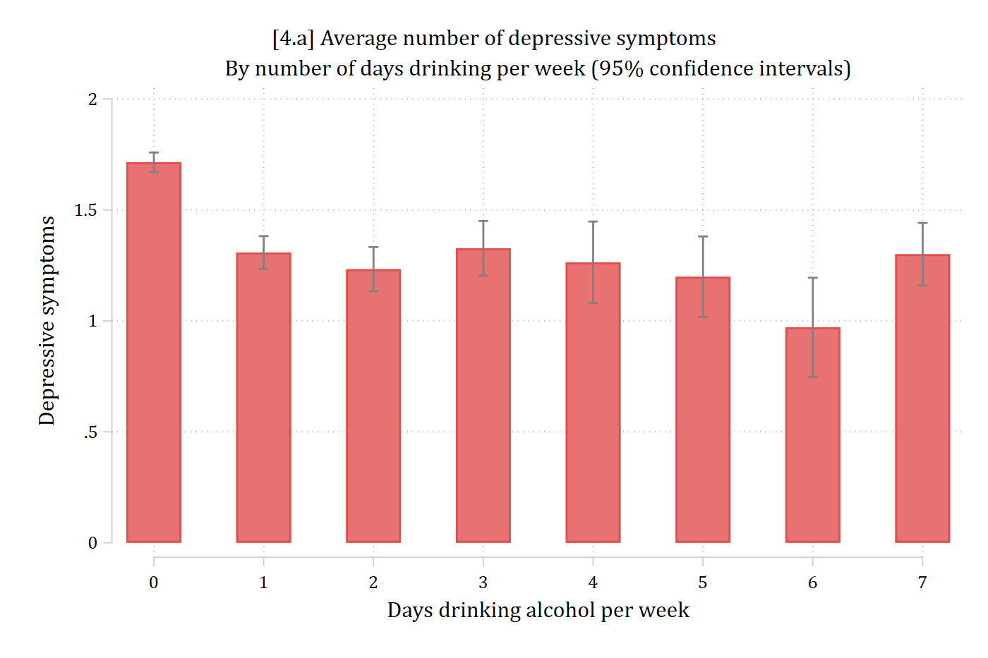
marginsplot, recast(bar) plotopts(barwidth(.5) col(*.7)) ciopts(col(gs8)) ///ytitle("Depressive symptoms") ylabel(0(0.5)2) ///xtitle("Days drinking alcohol per week") ///title("[4.a] Average number of depressive symptoms") ///subtitle("By number of days drinking per week (95% confidence intervals)")
Variables that uniquely identify means: dayweekdrink
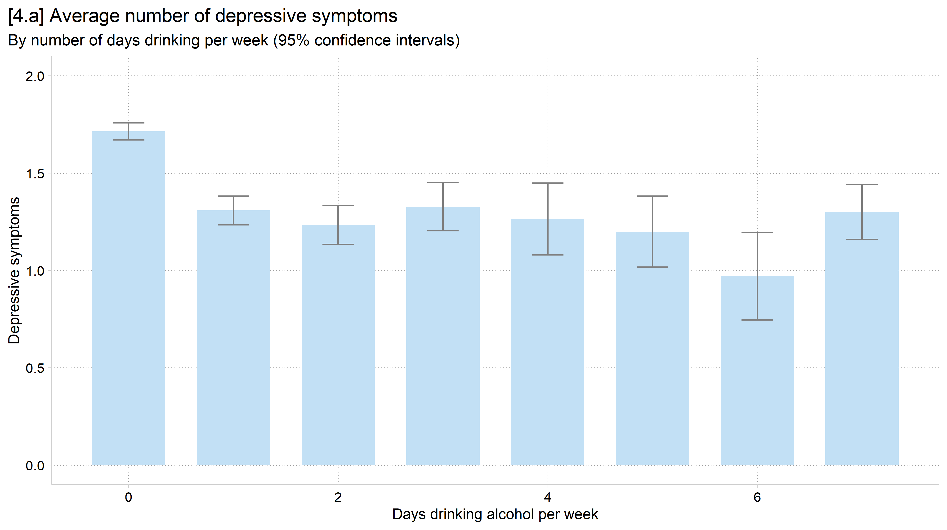
library(foreign) # load Stata datasetslibrary(ggplot2) # main graphics packagelibrary(dplyr) # data manipulation toolslibrary(cleanplots) # Mize's graphics scheme## Use cleanplots colors, markers, lines, and theme for all graphs ##cleanplots_defaults()theme_update(plot.title.position ="plot") # titles start at left edge of graph# Health and Retirement Study Datahrs <-read.dta("https://tdmize.github.io/data/data/hrs_si.dta")# 4.a - Add 95% confidence intervals to the bar chart (2022 wave)ggplot(filter(hrs, year ==2022), aes(x = dayweekdrink, y = cesd)) +stat_summary(fun = mean, geom ="bar", fill =cleanplots_colors("ltblue", bars =TRUE),width = .7) +stat_summary(fun.data = mean_cl_normal, geom ="errorbar", width = .3, color ="gray50") +labs(x ="Days drinking alcohol per week",y ="Depressive symptoms",title ="[4.a] Average number of depressive symptoms",subtitle ="By number of days drinking per week (95% confidence intervals)") +scale_y_continuous(breaks =seq(0, 2, 0.5)) +coord_cartesian(ylim =c(0, 2))
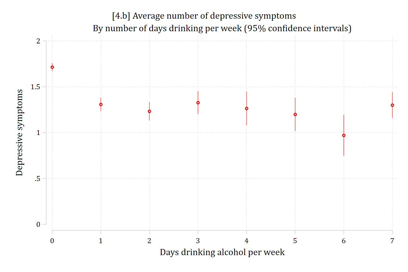
// 4.b - Recreate plot above but with a dot plotmarginsplot, recast(scatter) recastci(rspike) ciopt(col(*.5)) ///ytitle("Depressive symptoms") ylabel(0(0.5)2) ///xtitle("Days drinking alcohol per week") ///title("[4.b] Average number of depressive symptoms") ///subtitle("By number of days drinking per week (95% confidence intervals)")
Variables that uniquely identify means: dayweekdrink
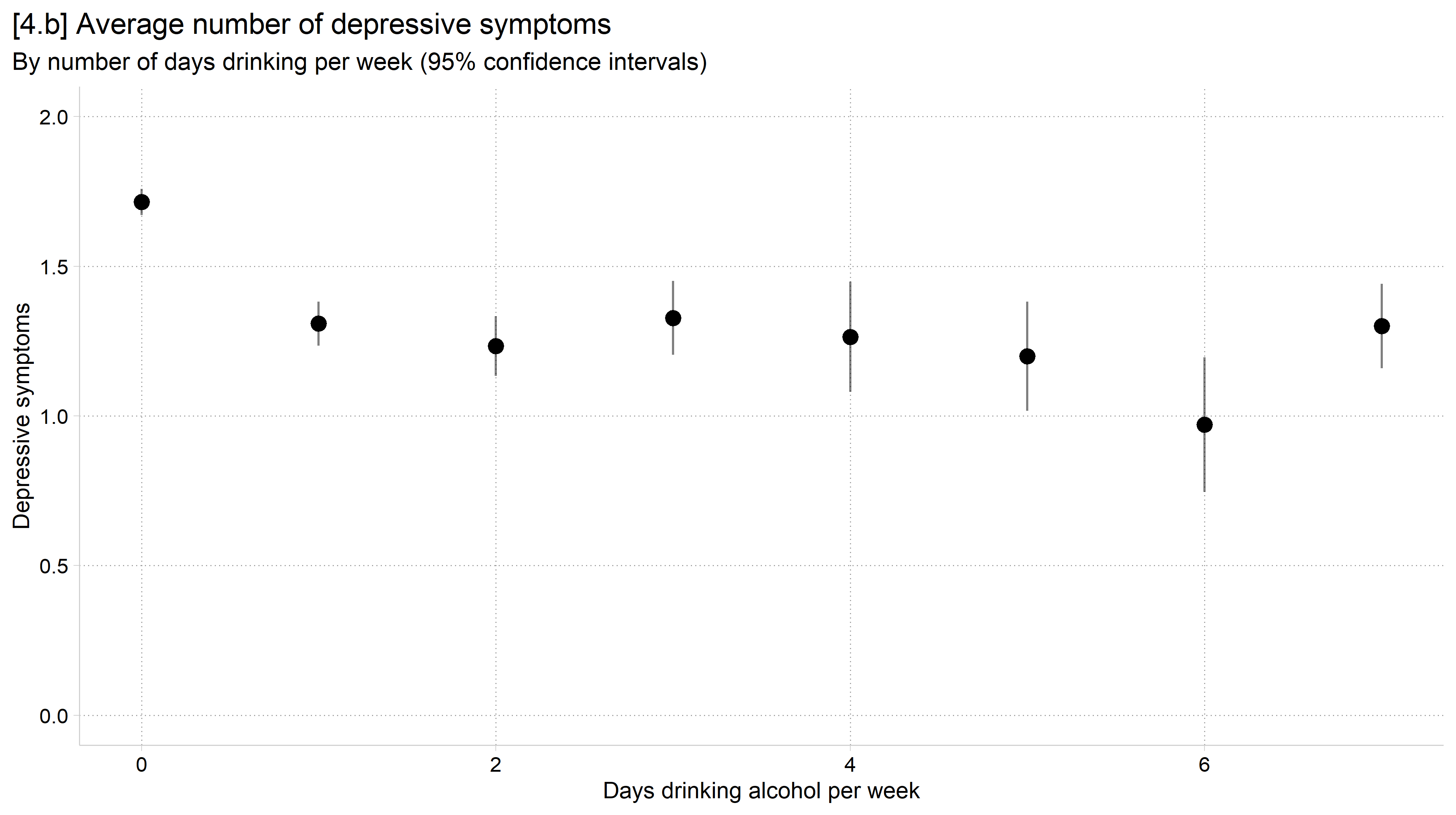
# 4.b - Recreate plot above but with a dot plotggplot(filter(hrs, year ==2022), aes(x = dayweekdrink, y = cesd)) +stat_summary(fun = mean, geom ="point", size =3) +stat_summary(fun.data = mean_cl_normal, geom ="linerange", alpha = .5) +labs(x ="Days drinking alcohol per week",y ="Depressive symptoms",title ="[4.b] Average number of depressive symptoms",subtitle ="By number of days drinking per week (95% confidence intervals)") +scale_y_continuous(breaks =seq(0, 2, 0.5)) +coord_cartesian(ylim =c(0, 2))
Bad graph levity
Moving forward: building blocks
“There is a strand of the data viz world that argues everything could be a bar chart. That’s possibly true but also possibly a world without joy.”(Amanda Cox, Editor, The Upshot, quoted in HBR 2013)
As we move into more advanced data and model visualizations the basic tools we learned in this section will often reappear
Aspects of both bar charts and dot plots are used very often in displaying complex model results
They both have good visualization properties and work nicely as the building blocks of more complicated graphs—where you can layer on additional aspects
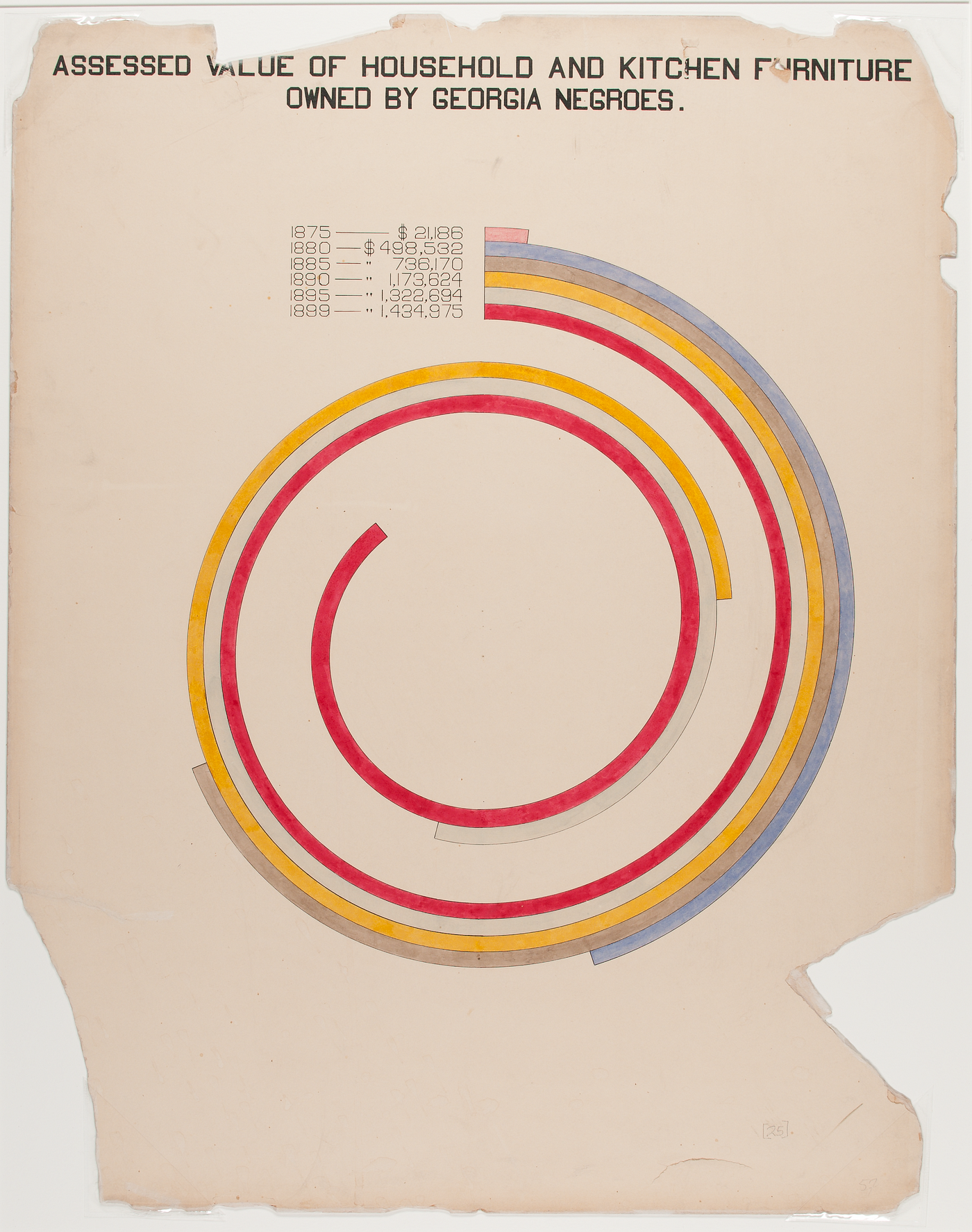
Bar chart that didn’t catch on
Read more about this spiral chart and other pioneering visualizations of W.E.B. DuBois