library(foreign); library(ggplot2); library(dplyr)

hrs <- read.dta("https://tdmize.github.io/data/data/hrs_si.dta")

ggplot(filter(hrs, !is.na(marstat), year == 2022),
       aes(x = marstat, y = lifesat)) +
  stat_summary(fun = mean, geom = "bar")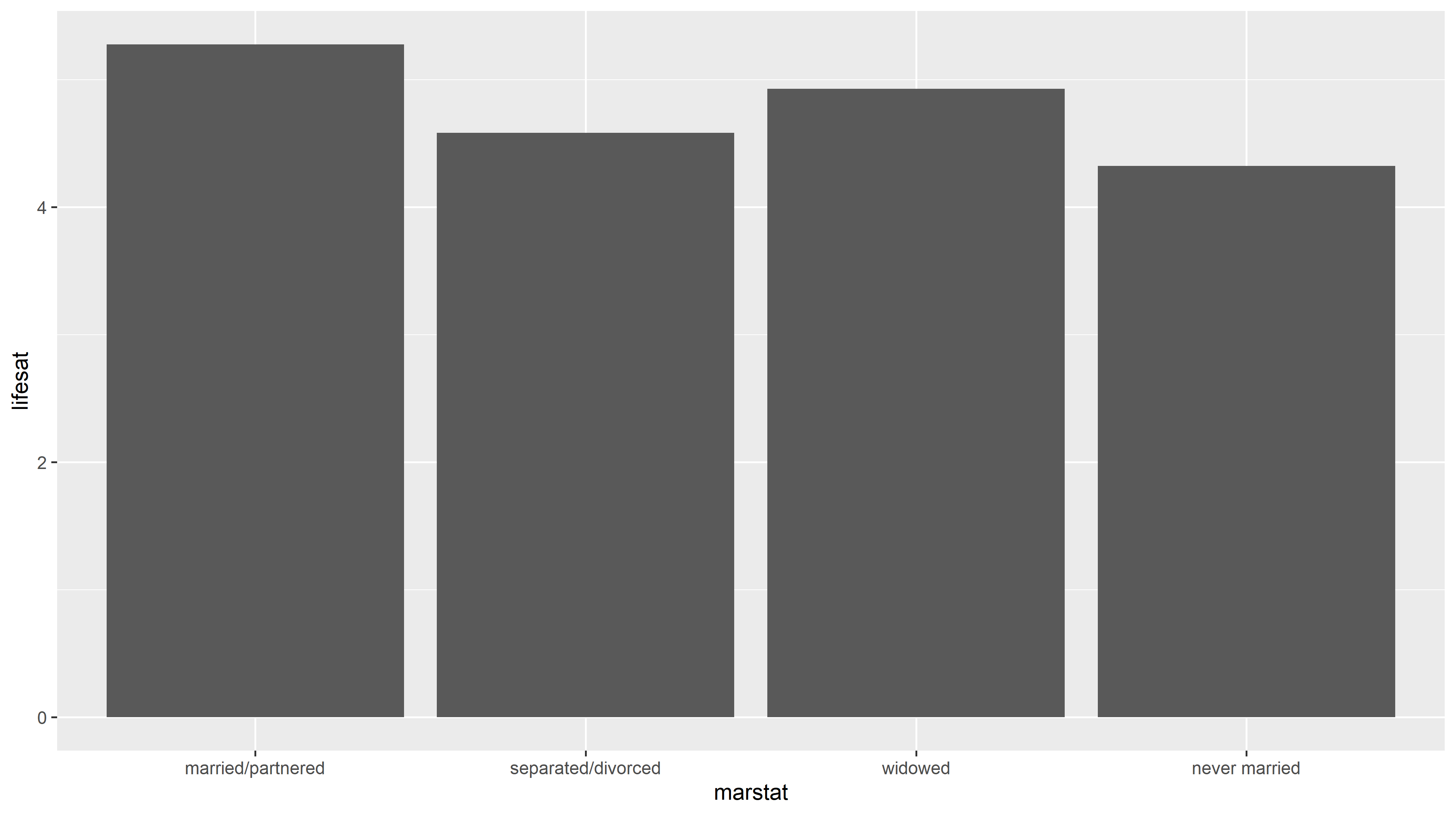
use "https://tdmize.github.io/data/data/hrs_si.dta", clear(Health and Retirement Study 1992-2022 - Cleaned for MCAP SI)graph bar (mean) lifesat if year == 2022, over(marstat)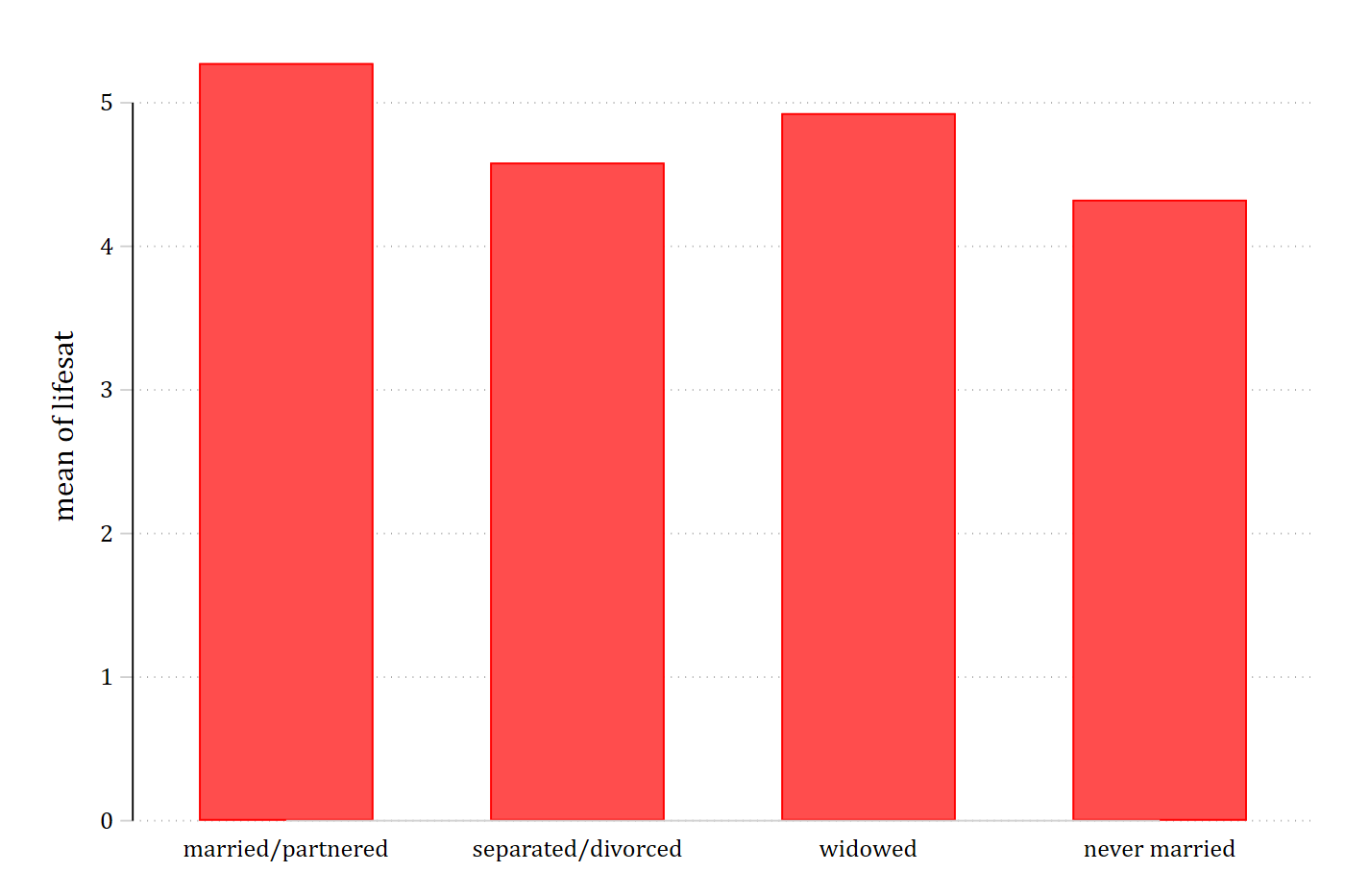
library(foreign); library(ggplot2); library(dplyr)
hrs <- read.dta("https://tdmize.github.io/data/data/hrs_si.dta")
ggplot(filter(hrs, !is.na(marstat), year == 2022),
aes(x = marstat, y = lifesat)) +
stat_summary(fun = mean, geom = "bar")
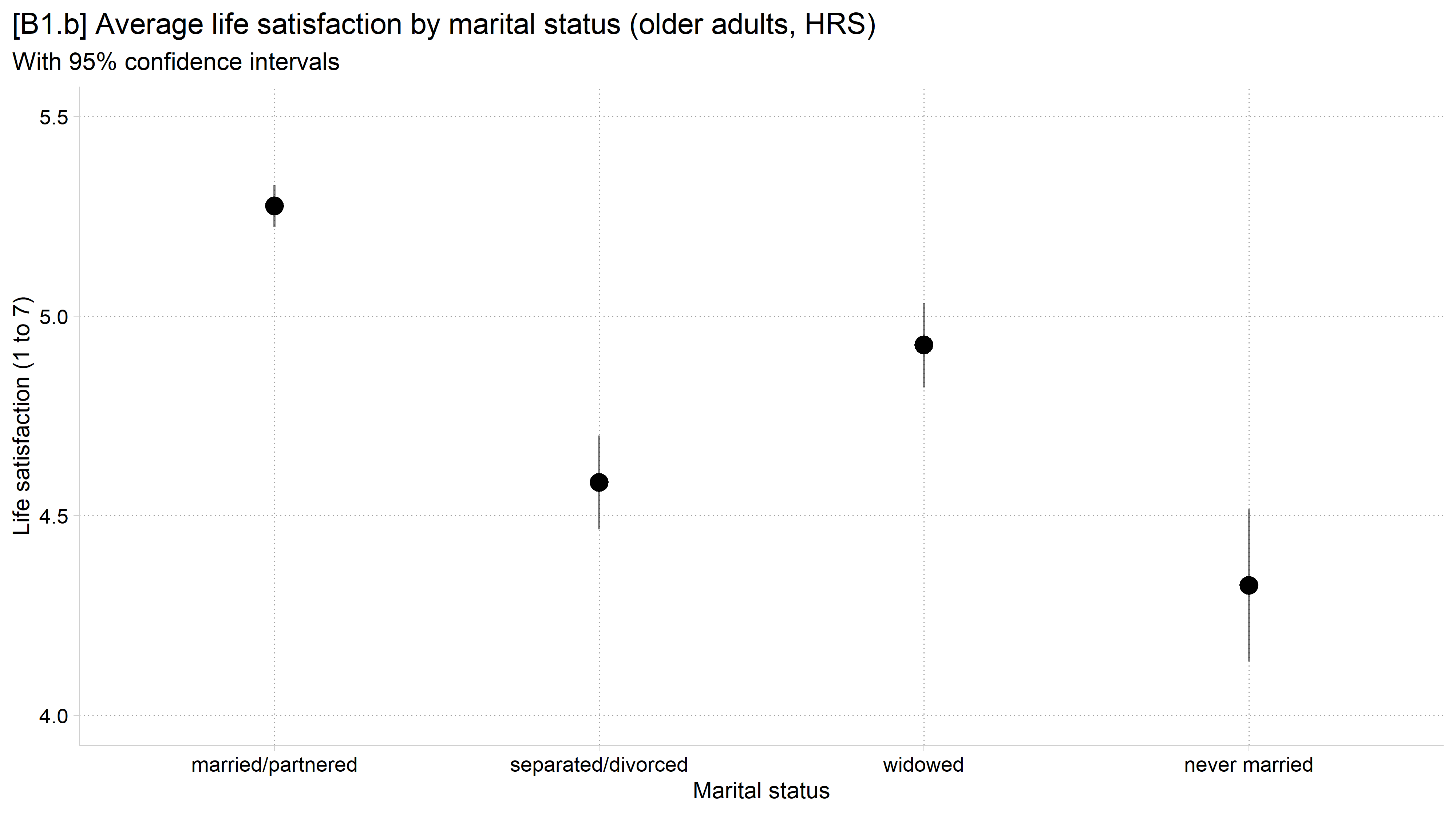
// B1.b - A publication-quality version
mean lifesat if year == 2022, over(marstat)
Mean estimation Number of obs = 4,410
---------------------------------------------------------------------
| Mean Std. err. [95% conf. interval]
--------------------+------------------------------------------------
c.lifesat@marstat |
married/partnered | 5.276 0.027 5.223 5.329
separated/divorced | 4.583 0.060 4.465 4.701
widowed | 4.927 0.054 4.821 5.034
never married | 4.325 0.097 4.135 4.515
---------------------------------------------------------------------coefplot, vertical msize(*1.2) ciopts(col(*.5)) ///
xlab(1 "married/partnered" 2 "separated/divorced" 3 "widowed" 4 "never mar
ried") ///
ytitle("Life satisfaction (1 to 7)") ylabel(4(.5)5.5) ///
xtitle("Marital status") ///
title("[B1.b] Average life satisfaction by marital status (older adults, H
RS)") ///
subtitle("With 95% confidence intervals")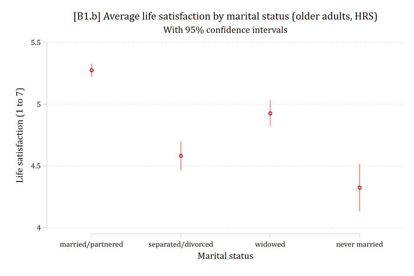
library(cleanplots)         # Mize's graphics scheme

## Use cleanplots colors, markers, lines, and theme for all graphs ##
cleanplots_defaults()
theme_update(plot.title.position = "plot")   # titles start at left edge of graph

# B1.b - A publication-quality version
ggplot(filter(hrs, !is.na(marstat), !is.na(lifesat), year == 2022),
       aes(x = marstat, y = lifesat)) +
  stat_summary(fun = mean, geom = "point", size = 3.6) +
  stat_summary(fun.data = mean_cl_normal, geom = "linerange", alpha = .5) +
  labs(x = "Marital status",
       y = "Life satisfaction (1 to 7)",
       title = "[B1.b] Average life satisfaction by marital status (older adults, HRS)",
       subtitle = "With 95% confidence intervals") +
  scale_y_continuous(breaks = seq(4, 5.5, .5)) + coord_cartesian(ylim = c(4, 5.5))