7.3 Nominal X Continuous Interactions

Why you should ignore the β coefficients when testing nonlinear interaction effects

use "https://tdmize.github.io/data/data/doan_love_SF", clear
(TESS03 - Analysis Dataset for TESS01 - Main Paper)
*Binary DV: support for legal marriage model
logit Bmarry i.cond##c.love10 rfem age rce_wht ed_coll ///
    ed_hs inc_50k married childyn children ideo evangel ///
    mainline blackprot catholic ofaithV2, or
Iteration 0:  Log likelihood = -304.06902  
Iteration 1:  Log likelihood = -185.27684  
Iteration 2:  Log likelihood = -171.23187  
Iteration 3:  Log likelihood = -169.29208  
Iteration 4:  Log likelihood = -169.22947  
Iteration 5:  Log likelihood =   -169.229  
Iteration 6:  Log likelihood =   -169.229  

Logistic regression                                     Number of obs =    501
                                                        LR chi2(20)   = 269.68
                                                        Prob > chi2   = 0.0000
Log likelihood = -169.229                               Pseudo R2     = 0.4435

-------------------------------------------------------------------------------
       Bmarry | Odds ratio   Std. err.      z    P>|z|     [95% conf. interval]
--------------+----------------------------------------------------------------
         cond |
         Gay  |      0.001      0.003   -2.841   0.005        0.000       0.125
     Lesbian  |      0.009      0.021   -1.995   0.046        0.000       0.920
              |
       love10 |      1.198      0.429    0.504   0.614        0.593       2.418
              |
cond#c.love10 |
         Gay  |      1.298      0.479    0.705   0.481        0.629       2.677
     Lesbian  |      1.009      0.373    0.025   0.980        0.489       2.084
              |
         rfem |      1.495      0.426    1.410   0.159        0.855       2.615
          age |      0.999      0.010   -0.138   0.891        0.979       1.018
      rce_wht |      1.144      0.446    0.346   0.730        0.533       2.457
      ed_coll |      0.877      0.458   -0.252   0.801        0.315       2.441
        ed_hs |      0.650      0.299   -0.936   0.349        0.264       1.601
      inc_50k |      0.973      0.324   -0.081   0.935        0.507       1.869
      married |      1.386      0.452    1.000   0.317        0.731       2.627
      childyn |      2.595      1.552    1.595   0.111        0.804       8.379
     children |      0.615      0.175   -1.706   0.088        0.352       1.075
         ideo |      0.542      0.063   -5.274   0.000        0.432       0.680
      evangel |      0.237      0.116   -2.946   0.003        0.091       0.618
     mainline |      0.684      0.354   -0.734   0.463        0.248       1.887
    blackprot |      0.230      0.151   -2.246   0.025        0.064       0.830
     catholic |      0.541      0.271   -1.227   0.220        0.203       1.443
     ofaithV2 |      0.819      0.591   -0.277   0.781        0.199       3.368
        _cons |   1376.326   3466.285    2.870   0.004        9.885    1.92e+05
-------------------------------------------------------------------------------
Note: _cons estimates baseline odds.
est store marry
library(haven)           # import Stata data and labels
library(dplyr)           # data manipulation
library(ggplot2)         # graphs
library(modelsummary)    # regression tables
library(marginaleffects) # predictions and marginal effects
library(cleanplots)      # graph scheme
cleanplots_defaults()

love <- read_dta("https://tdmize.github.io/data/data/doan_love_SF.dta")

# Keep model variables; drop any missing data
love <- love[c("Bmarry", "cond", "love10", "rfem", "age", "rce_wht", "ed_coll",
  "ed_hs", "inc_50k", "married", "childyn", "children", "ideo", "evangel",
  "mainline", "blackprot", "catholic", "ofaithV2")]
love <- love[complete.cases(love), ] |>
  mutate(cond = as_factor(cond))

# Binary DV: support for legal marriage model
marry <- glm(Bmarry ~ cond * love10 + rfem + age + rce_wht + ed_coll + ed_hs +
  inc_50k + married + childyn + children + ideo + evangel + mainline + blackprot +
  catholic + ofaithV2, data = love, family = binomial(link = "logit"))

modelsummary(marry, exponentiate = TRUE, stars = c("*" = .05, "**" = .01, "***" = .001),
  coef_omit = "rfem|age|rce_wht|ed_|inc_50k|married|child|ideo|evangel|mainline|blackprot|catholic|ofaith")
(1)
* p < 0.05, ** p < 0.01, *** p < 0.001
(Intercept) 1376.326**
(3466.182)
condGay 0.001**
(0.003)
condLesbian 0.009*
(0.021)
love10 1.198
(0.429)
condGay × love10 1.298
(0.479)
condLesbian × love10 1.009
(0.373)
Num.Obs. 501
AIC 380.5
BIC 469.0
Log.Lik. -169.229
F 5.010
RMSE 0.33
  • If we approached the interaction effect from this nonlinear model as we would for linear effects, the conclusion would be that: the effect of love is no different for gay and lesbian couples, compared to the effect of love for heterosexual couple

    This is wrong.

Plot the predictions

  • The presence of interaction terms in the model does not change the code for plotting predictions at all
  • In Stata, use margins for the predictions and marginsplot to make the graph
margins cond, at(love10=(0(0.5)10))

marginsplot
  • In R, use plot_predictions
plot_predictions(marry, by = c("love10", "cond"),
  newdata = datagrid(love10 = seq(0, 10, .5), cond = unique, grid_type = "counterfactual"))
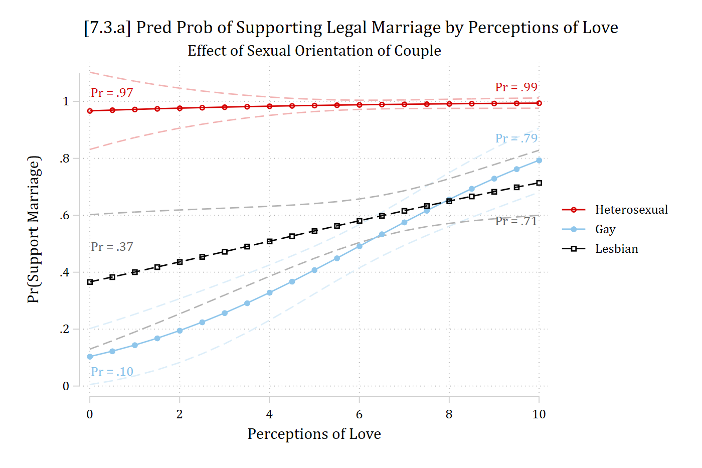
mtable, at(love10=(0 10) cond=(1 2 3)) decimals(2)
Expression: Pr(Bmarry), predict()

           |     cond    love10     Pr(y)
 ----------+-----------------------------
         1 |        1         0      0.97
         2 |        1        10      0.99
         3 |        2         0      0.10
         4 |        2        10      0.79
         5 |        3         0      0.37
         6 |        3        10      0.71

Specified values where .n indicates no values specified with at()

           |  No at()
 ----------+---------
   Current |       .n
*7.3.a
qui margins, at(love10=(0(0.5)10) cond=(1 2 3))
marginsplot, recastci(rline) ciopt(lpat(dash) lcol(*.3)) xlab(0(2)10) ylab(0(.
2)1.1) ///
    title("[7.3.a] Pred Prob of Supporting Legal Marriage by Perceptions of Lo
ve", size(medium)) ///
    subtitle("Effect of Sexual Orientation of Couple") ///
    ytitle("Pr(Support Marriage)") xtitle("Perceptions of Love") ///
    text(1.03 .5 "Pr = .97"  1.05 9.5 "Pr = .99", size(small) color(red*1.2)) 
///
    text(0.05 .5 "Pr = .10"  0.87 9.5 "Pr = .79", size(small) color(eltblue)) 
///
    text(0.49 .5 "Pr = .37"  0.58 9.5 "Pr = .71", size(small) color(gs6))
Variables that uniquely identify margins: love10 cond

[7.3.a] Predicted probability of supporting legal marriage by perceptions of love (0 to 10) for heterosexual, gay, and lesbian couples. Support for heterosexual couples is nearly flat near the top, from .97 to .99. Support for gay couples rises steeply from .10 to .79, and for lesbian couples from .37 to .71; the gay and lesbian lines cross near love = 8.

avg_predictions(marry, by = c("love10", "cond"),
  newdata = datagrid(love10 = c(0, 10), cond = unique, grid_type = "counterfactual"))

 love10         cond Estimate Std. Error      z Pr(>|z|)     S  2.5 % 97.5 %
      0 Heterosexual    0.967    0.06921  13.97   <0.001 144.9 0.8313  1.103
      0 Gay             0.104    0.05017   2.07   0.0389   4.7 0.0053  0.202
      0 Lesbian         0.366    0.12056   3.04   0.0024   8.7 0.1296  0.602
     10 Heterosexual    0.994    0.00917 108.42   <0.001   Inf 0.9762  1.012
     10 Gay             0.793    0.05736  13.83   <0.001 142.1 0.6809  0.906
     10 Lesbian         0.714    0.05824  12.26   <0.001 112.4 0.6001  0.828

Type: response
# 7.3.a
plot_predictions(marry, by = c("love10", "cond"),
  newdata = datagrid(love10 = seq(0, 10, .5), cond = unique, grid_type = "counterfactual")) +
  annotate("text", x = c(.5, 9.5, .5, 9.5, .5, 9.5), y = c(1.03, 1.05, .05, .87, .49, .58),
    label = c("Pr = .97", "Pr = .99", "Pr = .10", "Pr = .79", "Pr = .37", "Pr = .71"),
    size = 3) +
  scale_x_continuous(breaks = seq(0, 10, 2)) +
  scale_y_continuous(breaks = seq(0, 1, .2)) +
  coord_cartesian(ylim = c(0, 1.1)) +
  labs(title = "[7.3.a] Pred Prob of Supporting Legal Marriage by Perceptions of Love",
    subtitle = "Effect of Sexual Orientation of Couple",
    x = "Perceptions of Love", y = "Pr(Support Marriage)", color = NULL, fill = NULL)

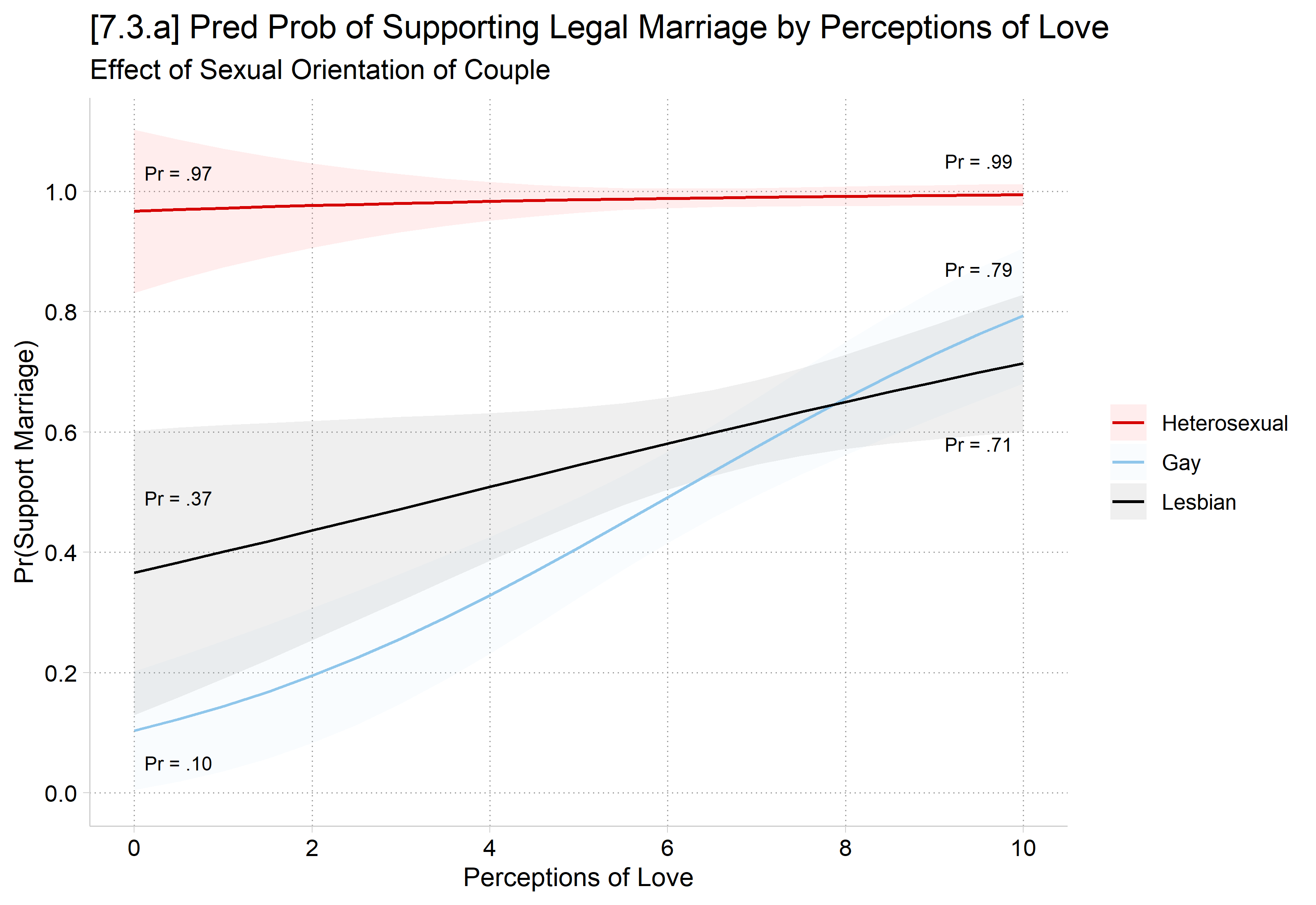
[7.3.a] Predicted probability of supporting legal marriage by perceptions of love (0 to 10) for heterosexual, gay, and lesbian couples. Support for heterosexual couples is nearly flat near the top, from .97 to .99. Support for gay couples rises steeply from .10 to .79, and for lesbian couples from .37 to .71; the gay and lesbian lines cross near love = 8.

Calculating 2nd differences in Stata and R

// MEs (1st differences) with mecompare.
**Focal IV goes in varlist; moderating variable in by( )
mecompare love10, by(cond) model(marry)
Predicting: Pr(Bmarry)
Marginal effects (N_marry=501)

                                 |  ME #   Estimate         SE      P>|z|
---------------------------------+---------------------------------------
love10 + 1 (centered)            |                                       
                    Heterosexual |     1      0.002      0.006      0.690
                             Gay |     2      0.071      0.012      0.000
                         Lesbian |     3      0.033      0.015      0.032
  • Use metest for the 2nd difference: equality of any two MEs (1st differences)
    • Refer to ME # from mecompare table
*use metest for 2nd difference: equality of any two MEs
metest 2 - 1
                                 |  estimate         se     pvalue 
---------------------------------+--------------------------------
   love10_cond_2 - love10_cond_1 |     0.068      0.013      0.000 
  • Can accumulate tests into a single table with metest
*Accumulate all 2nd diffs into a single metest table
metest, clear
qui metest 2 - 1, add rowname("Gay - Hetero")
qui metest 3 - 1, add rowname("Lesbian - Hetero")
qui metest 2 - 3, add rowname("Gay - Lesbian")
metest, title("2nd difference of effect of love, by couple type")
2nd difference of effect of love, by couple type

                                 |  estimate         se     pvalue 
---------------------------------+--------------------------------
                    Gay - Hetero |     0.068      0.013      0.000 
                Lesbian - Hetero |     0.031      0.017      0.063 
                   Gay - Lesbian |     0.037      0.019      0.049 
  • In R, use avg_comparisons to calculate the MEs (1st differences)
# Changes in continuous IVs centered on the observed values, like mecompare
options(marginaleffects_contrast_direction = "center")

# MEs (1st differences)
avg_comparisons(marry, variables = "love10", by = "cond",
  newdata = datagrid(cond = unique, grid_type = "counterfactual"))

         cond Estimate Std. Error     z Pr(>|z|)    S    2.5 % 97.5 %
 Heterosexual  0.00235    0.00589 0.399   0.6897  0.5 -0.00920 0.0139
 Gay           0.07065    0.01189 5.944   <0.001 28.4  0.04735 0.0939
 Lesbian       0.03319    0.01549 2.143   0.0321  5.0  0.00284 0.0635

Term: love10
Type: response
Comparison: +1
  • Add a hypothesis option to test for 2nd difference (the equality of any two MEs)
    • MEs named b# in order they appear in avg_comparisons output from last step
avg_comparisons(marry, variables = "love10", by = "cond",
  newdata = datagrid(cond = unique, grid_type = "counterfactual"),
  hypothesis = "b2 - b1 = 0")

 Hypothesis Estimate Std. Error    z Pr(>|z|)    S  2.5 % 97.5 %
    b2-b1=0   0.0683     0.0132 5.18   <0.001 22.1 0.0424 0.0941

Type: response
  • The hypothesis option ~pairwise will calculate all 2nd differences
avg_comparisons(marry, variables = "love10", by = "cond",
  newdata = datagrid(cond = unique, grid_type = "counterfactual"),
  hypothesis = ~ pairwise)

                 Hypothesis Estimate Std. Error     z Pr(>|z|)    S    2.5 %    97.5 %
 (Gay) - (Heterosexual)       0.0683     0.0132  5.18   <0.001 22.1  0.04245  0.094139
 (Lesbian) - (Heterosexual)   0.0308     0.0166  1.86   0.0626  4.0 -0.00163  0.063298
 (Lesbian) - (Gay)           -0.0375     0.0190 -1.97   0.0491  4.3 -0.07477 -0.000146

Type: response

The effect of love is stronger for gay couples than for heterosexual couples, indicating an interaction effect (2nd diff. = 0.068, p < .001).

Etc.

See additional example interpretations under “Example write-up” below

Plotting the “other side” of the interaction

  • Conceptually, it is useful to specify a focal IV and a moderating IV
    • This is mostly a theoretical distinction, but can influence the test with nonlinearities
  • Usually, the variable that comes first in your research question/hypothesis is the focal IV; the variable whose effect it (may) vary across is the moderating IV

RQ ex: Do perceptions of love have different effects for varying couple types?

H ex: Perceptions of love should have a stronger effect for gay couples compared to its effect for heterosexual couples.

RQ ex: Does aging lead to declining physical health at equal rates for individuals from different racial-ethnic backgrounds?

H ex: Aging will have a stronger (more negative) effect on physical health for Black than for White adults.

  • The examples above focus mostly on the effect of love as the focal IV, and couple type as the moderating IV
  • It is also important to examine the effect of the moderating IV, across values of the focal IV
    • Essentially, flip the focal and moderating variable
  • For a continuous X nominal interaction: calculate the marginal effect (ME) of the nominal IV across the range of the continuous IV and plot it
    • Note for this example because our nominal IV has 3 categories we have to pick a reference category and then plot two lines which are the differences from the reference
  • In Stata, calculate ME of nominal IV across range of continuous IV using margins
    • Plot with marginsplot
*7.3.b - Effect of sexual orientation (heterosexual vs [gay & lesbian])
*   over range of love
est restore marry
(results marry are active now)
qui margins, dydx(cond) at(love=(0(0.5)10))
marginsplot, recastci(rline) ci1opts(lpat(dash) col(eltblue*.4)) ///
    ci2opts(lpat(dash) col(gs10*.4)) ///
    plot1op(lcol(eltblue) msym(none) lwid(medthick)) ///
    plot2op(lcol(gs10) msym(none) lwid(medthick)) ///
    ylab(-1(0.2)0.2) xlab(0(1)10) yline(0, lcol(black)) ///
    title("[7.3.b] Difference in Support for Marriage: Gay/Lesbian vs Heterose
xual Couple", size(medsmall)) ///
    subtitle("Effects Below Zero Indicate Lower Support for Gay/Lesbian Couple
's Marriage Rights", size(small)) ///
    ytitle("Pr(Support): Gay/Lesbian - Heterosexual") ///
    legend(order(3 "Gay vs Hetero" 4 "Lesbian vs Hetero") pos(6) row(1))
Variables that uniquely identify margins: love10 _deriv

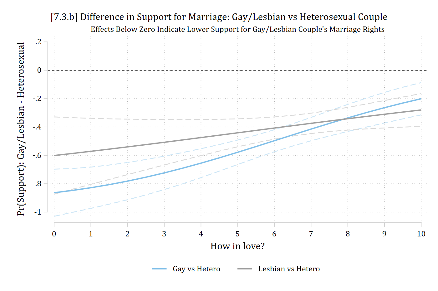
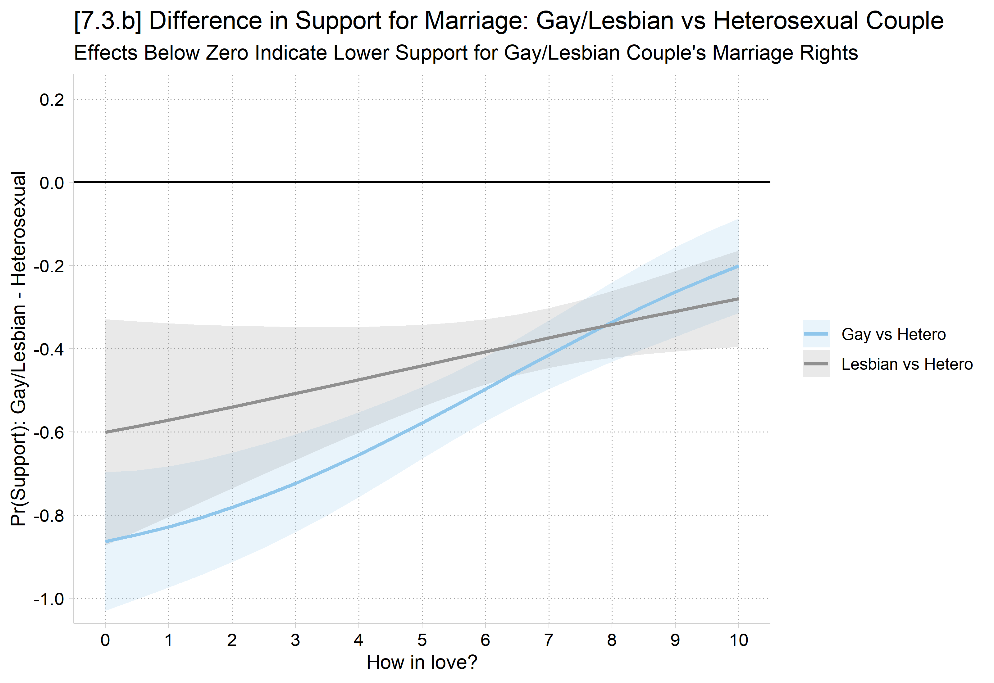
[7.3.b] Marginal effect of couple type (gay vs heterosexual and lesbian vs heterosexual) on the probability of supporting marriage, across perceptions of love from 0 to 10, with confidence intervals and a line at zero. Both differences are negative throughout: the gay vs heterosexual difference rises from about -0.87 at love = 0 to about -0.2 at love = 10, and the lesbian vs heterosexual difference rises from about -0.6 to about -0.28; the lines cross near love = 8.

  • In R, use plot_comparisons
# 7.3.b - Effect of sexual orientation (heterosexual vs [gay & lesbian])
#   over range of love (MEs saved and passed to ggplot to draw both lines in one panel)
mes <- avg_comparisons(marry, variables = "cond", by = c("love10", "contrast"),
  newdata = datagrid(love10 = seq(0, 10, .5), grid_type = "counterfactual"))

ggplot(mes, aes(x = love10, y = estimate, color = contrast, fill = contrast)) +
  geom_ribbon(aes(ymin = conf.low, ymax = conf.high), alpha = .2, color = NA) +
  geom_line(linewidth = 1) +
  geom_hline(yintercept = 0) +
  scale_color_manual(values = c("#8FC6EB", "#909090"),
    labels = c("Gay vs Hetero", "Lesbian vs Hetero")) +
  scale_fill_manual(values = c("#8FC6EB", "#909090"),
    labels = c("Gay vs Hetero", "Lesbian vs Hetero")) +
  scale_x_continuous(breaks = 0:10) +
  scale_y_continuous(breaks = seq(-1, .2, .2)) +
  coord_cartesian(ylim = c(-1, .2)) +
  labs(title = "[7.3.b] Difference in Support for Marriage: Gay/Lesbian vs Heterosexual Couple",
    subtitle = "Effects Below Zero Indicate Lower Support for Gay/Lesbian Couple's Marriage Rights",
    x = "How in love?", y = "Pr(Support): Gay/Lesbian - Heterosexual", color = NULL, fill = NULL)

[7.3.b] Marginal effect of couple type (gay vs heterosexual and lesbian vs heterosexual) on the probability of supporting marriage, across perceptions of love from 0 to 10, with confidence intervals and a line at zero. Both differences are negative throughout: the gay vs heterosexual difference rises from about -0.87 at love = 0 to about -0.2 at love = 10, and the lesbian vs heterosexual difference rises from about -0.6 to about -0.28; the lines cross near love = 8.

*Recall this is a direct test of gay vs heterosexual couple: if the 95% confidence interval does not overlap zero: the group difference is statistically significant at p < 0.05

Example write-up

Perceptions of how in love a couple is have differential effects on how supportive someone is of legal marriage rights, depending on the sexual orientation of the couple. For heterosexual couples, perceptions of love have no effect on support for marriage (∆heterosexual p = ns). This is because heterosexual couples receive overwhelming support for legal marriage regardless of whether someone sees them as not in love at all (Pr = 0.97) or whether they see them as extremely in love (Pr = 0.99; see red line in Figure 1). Perceptions of love have a relatively small but significant effect on support for marriage of lesbian couples (∆lesbian = 0.033 p < 0.05). There is a large positive effect of love for gay couples (∆gay = 0.071 p < 0.001). For example, support for legal marriage rises drastically over the range of love, from a low of just 0.10 to a high of 0.79 for gay couples who are viewed as extremely in love (see blue line in Figure 1). The effect of love is stronger for gay men than for heterosexual couples (2nd difference = 0.068; p < 0.001) and for gay men compared to lesbian couples (2nd difference = 0.037; p < 0.05). However, it is important to note that despite the strong increase in support for marriage for gay couples as perceptions of love increase, support for a gay couple’s marriage rights is never equal to support for heterosexual couple’s marriage rights (see Figure 2).

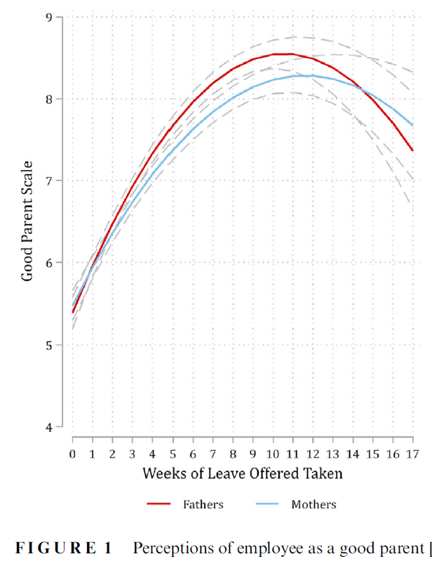
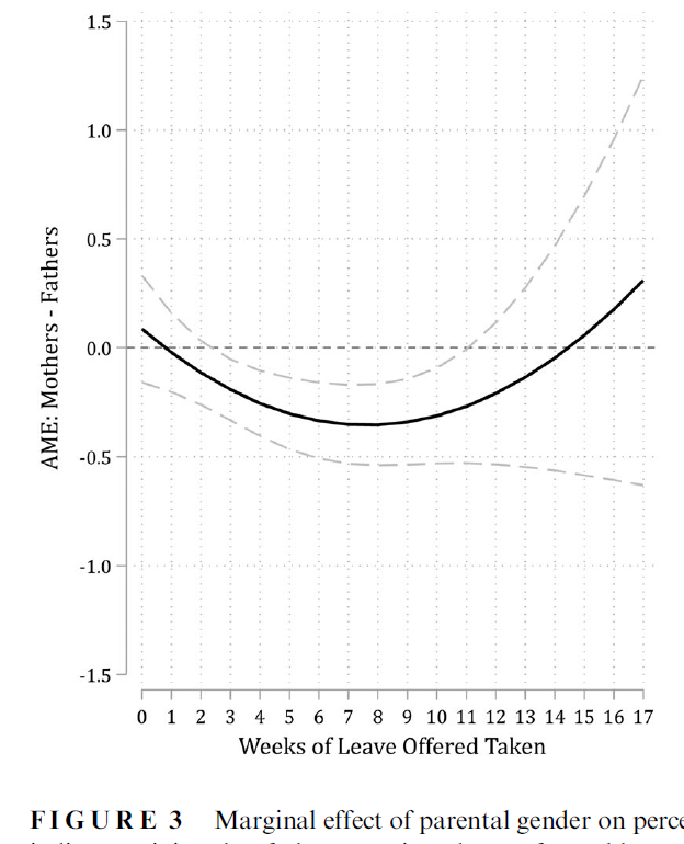
Figure 1 from Petts, Kaufman, and Mize (2023): perceptions of an employee as a good parent by weeks of leave offered, for fathers and mothers. Both curves rise and then fall, peaking around 9 to 11 weeks. Figure 3 from Petts, Kaufman, and Mize (2023): the marginal effect of parental gender (mothers minus fathers) across weeks of leave offered, with confidence intervals and a line at zero. The effect dips slightly below zero in the middle weeks and rises above zero at the longest leaves.

*I like including both graphs in a single paper (often as separate panels) to help the reader follow what the second graph shows. Example from Petts, Kaufman, and Mize 2023
Back to top