5.1 Latent Variable Model

Structural model relating x’s to y*

The structural model can be conceptualized in an identical fashion to the binary regression model
In a latent variable y* formulation—substantively—we are assuming a latent continuous dependent variable y* exists and that someone’s place on y* is the cause of their observed category choice y
- Our data only has partial information: the categorical (ordinal) y
The structural model:

\[y^{*} = \mathbf{x}_{i}\boldsymbol{\beta} + \varepsilon\]

Measurement model linking y* to y

Just as in binary regression, we don’t observe y*
- With ordinal DVs we observe an ordinal variable y with J total categories
  - Each individual category = j

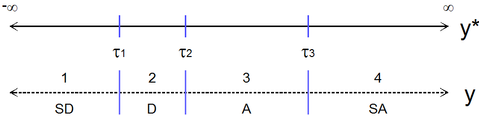
A latent y-star line from minus infinity to infinity split by three thresholds tau 1, tau 2, and tau 3 into four observed categories of y: 1 SD, 2 D, 3 A, and 4 SA.

Observed y is theoretically obtained from y* by dividing it into segments by thresholds τ_j (tau)

\[y_{i} = j \quad \text{if} \quad \tau_{j-1} \leq y_{i}^{*} < \tau_{j}\]

\[y_{i} = \begin{cases} 1 \Rightarrow \text{SD-Strongly Disagree} & \text{if } \tau_{0} = -\infty \leq y_{i}^{*} < \tau_{1} \\ 2 \Rightarrow \text{D-Disagree} & \text{if } \tau_{1} \leq y_{i}^{*} < \tau_{2} \\ 3 \Rightarrow \text{A-Agree} & \text{if } \tau_{2} \leq y_{i}^{*} < \tau_{3} \\ 4 \Rightarrow \text{SA-Strongly Agree} & \text{if } \tau_{3} \leq y_{i}^{*} < \tau_{4} = \infty \end{cases}\]

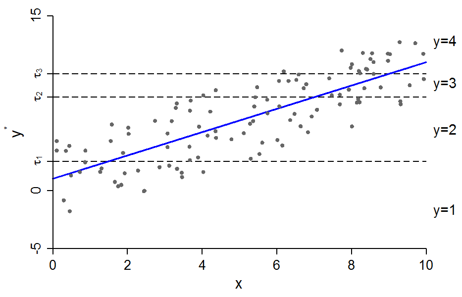
Scatterplot of latent y-star against x from 0 to 10 with a rising regression line; three dashed horizontal lines at the thresholds tau 1, tau 2, and tau 3 divide the points into the observed categories y = 1 to y = 4.

Conceptually, imagine we measured the true latent variable (y*) and then decided later to collapse the continuous variable into four ordered categories

Since y* is latent we focus on Pr(y = j | x)

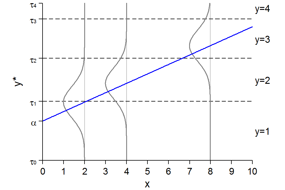
Latent y-star rising linearly with x, with normal error distributions drawn at x = 2, 4, and 8; dashed lines at the thresholds tau 1, tau 2, and tau 3 split each distribution into the probabilities of y = 1 to y = 4.

Conceptually, y* is responsible for the observed categories of y. Remember we don’t actually observe y* (so we can’t directly estimate slope of the blue line). Instead, we need to take the information we do have on the proportion of responses in each category of y, make some assumptions, and extrapolate to y* (and thus the blue line)

Assumptions & predicted probabilities for ordered models

A latent y-star line split by thresholds tau 1, tau 2, and tau 3 into four observed categories of y: 1 SD, 2 D, 3 A, and 4 SA.

To get predictions, we examine whether predicted y* is between thresholds
- Example: y = 2 when y* is between τ₁ and τ₂

\[\Pr(y = 2\,|\,\mathbf{x}) = \Pr(\tau_{1} \leq y^{*} < \tau_{2}\,|\,\mathbf{x})\]

Expanding y*

\[\Pr(y = 2\,|\,\mathbf{x}) = \Pr(\tau_{1} \leq \alpha + \beta x + \varepsilon < \tau_{2}\,|\,\mathbf{x})\]

We need some additional assumptions about α and ε to identify the model (below)

Identification

Because y* is unobserved we do not know its scale. To set the scale of y* and to compute Pr(y = j | x) we need to make some assumptions which affect the scale/metric of the DV:
- Ordered probit assumes: \(\varepsilon \sim N(0, 1)\)
- Ordered logit assumes: \(\varepsilon \sim \lambda(0, \pi^{2}/3)\)
We cannot estimate all of the thresholds* and the intercept
- One of two sets of identifying assumptions are often used
  
  Alternative 1: \(\tau_{1} = 0\)
  
  Alternative 2: \(\alpha = 0\)
These alternatives lead to different parameterizations. But the parameterization chosen:
- Does not affect the βs
- Does not affect the significance tests of the βs
- Does not affect the predicted probabilities of specific outcomes

*Note only J – 1 thresholds are needed (refer back to the continuum above; how many thresholds needed to know which category an observation is in?)

Potential software issues

Numerical methods for maximum likelihood estimation are readily available, although in practice the ordinal model can be a difficult model for obtaining convergence
- Generally, takes longer to converge than most other categorical DV models
Different software packages will use different parameterizations
Small n’s in a category can lead to failure to converge
- You can merge adjacent categories and only lose information… if the model assumptions are correct!

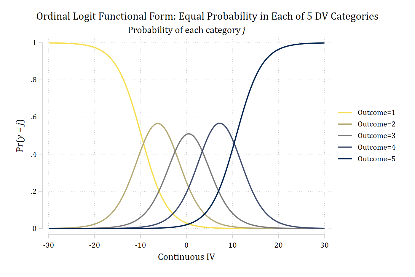
Ordinal logit functional form with five equally likely categories: Pr(outcome 1) falls and Pr(outcome 5) rises across the continuous IV, with hill-shaped curves for outcomes 2, 3, and 4 in between.

(The code for this graph is in 5.0)

Merging adjacent categories

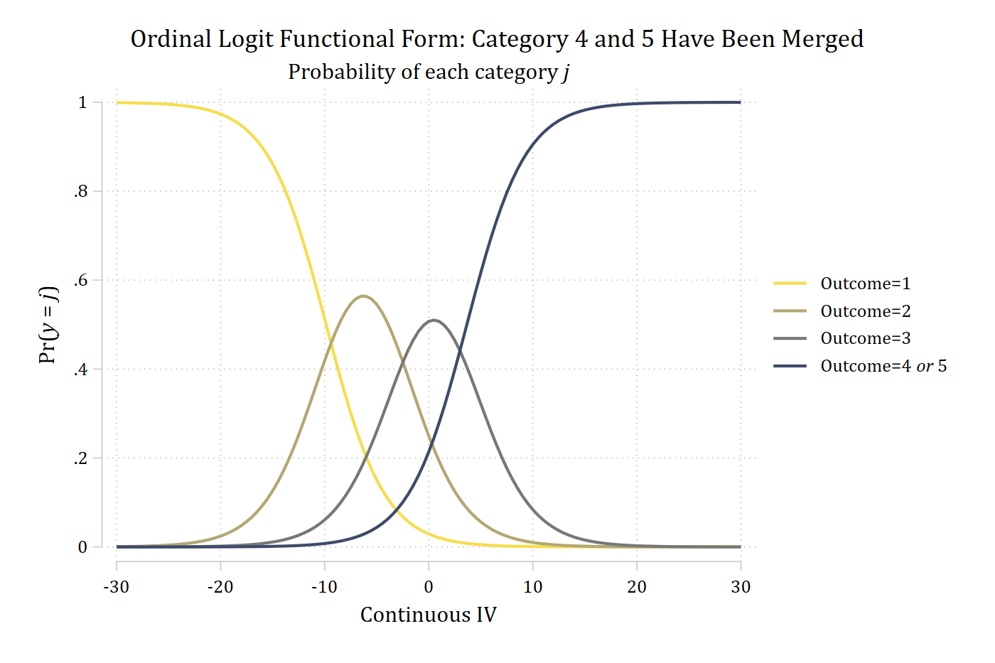
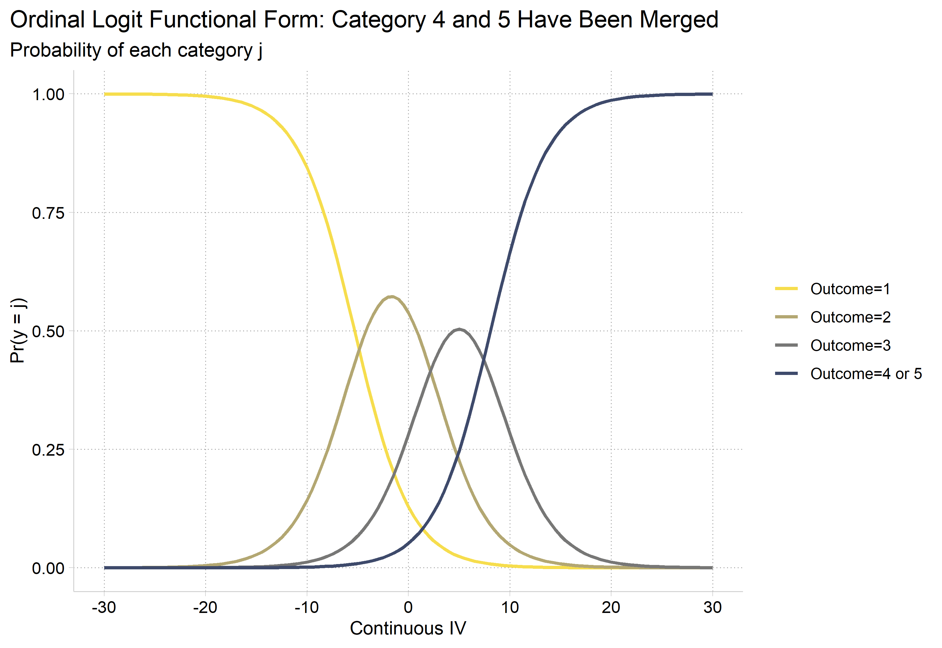
Our observed y above has 5 categories. We can merge categories 4 and 5 and lose some information but not our ability to estimate the model
- Critically, our estimates in terms of y* should be identical regardless as to whether we use all 5 categories or just the 4
- However, we lose the ability with the 4 category DV to separately examine the Pr(y = 4) and the Pr(y = 5)

* Simulated data from 5.0 (see the code there)
// Merge categories to demonstrate only lose info
gen y_merge_4_5 = y
recode y_merge_4_5 4 5 = 4

(400 changes made to y_merge_4_5)

tab y y_merge_4_5

         5 |
 quantiles |                 y_merge_4_5
  of ystar |         1          2          3          4 |     Total
-----------+--------------------------------------------+----------
         1 |       400          0          0          0 |       400 
         2 |         0        400          0          0 |       400 
         3 |         0          0        400          0 |       400 
         4 |         0          0          0        400 |       400 
         5 |         0          0          0        400 |       400 
-----------+--------------------------------------------+----------
     Total |       400        400        400        800 |     2,000

// Equal distribution in each outcome category //
qui ologit y_merge_4_5 c.c i.b x1 x2
*Pr(probs)
qui margins, at(c=(-30(.5)30)) atmeans
marginsplot, noci plotopts(msym(none) lwidth(medthick) lpat(solid)) ///
    xlab(-30(10)30) xtitle("Continuous IV") ytitle("Pr({it:y} = {it:j})") ///
    title("Ordinal Logit Functional Form: Category 4 and 5 Have Been Merged", 
size(medium)) ///
    subtitle("Probability of each category {it:j}") ///
    legend(order(1 "Outcome=1" 2 "Outcome=2" 3 "Outcome=3" 4 "Outcome=4 {it:or
} 5")) ///
    scheme(cleanplots5)

Variables that uniquely identify margins: c

Ordinal logit functional form after merging categories 4 and 5: the curves for outcomes 1, 2, and 3 are the same as with five categories, and the merged outcome 4 or 5 rises from 0 to about 1 across the continuous IV.

# Simulated data from 5.0 (see the code there)

# Merge categories to demonstrate only lose info
sim <- sim |>
  mutate(y_merge_4_5 = factor(ifelse(as.numeric(y) >= 4, 4, as.numeric(y))))
table(sim$y, sim$y_merge_4_5)

   
      1   2   3   4
  1 400   0   0   0
  2   0 400   0   0
  3   0   0 400   0
  4   0   0   0 400
  5   0   0   0 400

# Equal distribution in each outcome category
mergemod <- polr(y_merge_4_5 ~ c + b + x1 + x2, data = sim, Hess = TRUE)

# Pr(probs) with the other IVs at their means
pr_merge <- predictions(mergemod, newdata = datagrid(c = seq(-30, 30, .5)))

ggplot(pr_merge, aes(x = c, y = estimate, color = group)) +
  geom_line(linewidth = 1) +
  scale_color_manual(values = viridisLite::cividis(5, end = .95, direction = -1)[1:4],
    labels = c("Outcome=1", "Outcome=2", "Outcome=3", "Outcome=4 or 5")) +
  scale_x_continuous(breaks = seq(-30, 30, 10)) +
  labs(title = "Ordinal Logit Functional Form: Category 4 and 5 Have Been Merged",
    subtitle = "Probability of each category j",
    x = "Continuous IV", y = "Pr(y = j)", color = NULL) +
  theme(plot.title.position = "plot")

Ordinal logit functional form after merging categories 4 and 5: the curves for outcomes 1, 2, and 3 are the same as with five categories, and the merged outcome 4 or 5 rises from 0 to about 1 across the continuous IV.