7.5 Continuous X Continuous Interactions

*GSS 1972 - 2024
use "https://tdmize.github.io/data/data/cda_gss24", clear
(GSS 1972-2024 CDA - Categorical Data Analysis | 2024-12-03)
*Drop any missing data on model vars
drop if missing(sameokB, year1972, conviewSS, age, race3, ///
    woman, faminc, married, college)
(37,893 observations deleted)
fre sameokB
sameokB -- Same-sex relationships not wrong at all
------------------------------------------------------------------------
                           |      Freq.    Percent      Valid       Cum.
---------------------------+--------------------------------------------
Valid   0 sometimes wrong  |      25726      68.05      68.05      68.05
        1 not wrong at all |      12080      31.95      31.95     100.00
        Total              |      37806     100.00     100.00           
------------------------------------------------------------------------
library(haven)           # import Stata data and labels
library(dplyr)           # data manipulation
library(ggplot2)         # graphs
library(sjmisc)          # frequency tables
library(marginaleffects) # predictions and marginal effects
library(cleanplots)      # graph scheme
cleanplots_defaults()

# GSS 1972 - 2024
gss <- read_dta("https://tdmize.github.io/data/data/cda_gss24.dta")

# Keep model variables; drop any missing data
gss <- gss[c("sameokB", "year1972", "conviewSS", "age", "race3", "woman", "faminc",
  "married", "college")]
gss <- gss[complete.cases(gss), ]

frq(gss, sameokB)
Same-sex relationships not wrong at all (sameokB) <numeric> 
# total N=37806 valid N=37806 mean=0.32 sd=0.47

Value |            Label |     N | Raw % | Valid % | Cum. %
-----------------------------------------------------------
    0 |  sometimes wrong | 25726 | 68.05 |   68.05 |  68.05
    1 | not wrong at all | 12080 | 31.95 |   31.95 | 100.00
 <NA> |             <NA> |     0 |  0.00 |    <NA> |   <NA>

Ideal types

  • Earlier in the class, we defined ideal types by clusters of multiple IVs
  • Can also think of ideal typical values for specific IVs
  • E.g., Say you were in charge of casting for a movie and the script calls for a “young person”, a “middle aged person”, and an “older person”
    • What age would you target for each role?
      • This is your ideal type / prototypical value

Cartoon faces of people of many ages, from babies and children to young adults and gray-haired older adults.

Ideal types example

fre conviewSS
conviewSS -- Lib to Cons politics scale
---------------------------------------------------------------------------
                              |      Freq.    Percent      Valid       Cum.
------------------------------+--------------------------------------------
Valid   1   Most liberal      |        772       2.04       2.04       2.04
        1.5                   |       1953       5.17       5.17       7.21
        2                     |       2566       6.79       6.79      14.00
        2.5                   |       4298      11.37      11.37      25.36
        3                     |       5235      13.85      13.85      39.21
        3.5                   |       4033      10.67      10.67      49.88
        4   Middle            |       4666      12.34      12.34      62.22
        4.5                   |       2857       7.56       7.56      69.78
        5                     |       3807      10.07      10.07      79.85
        5.5                   |       2912       7.70       7.70      87.55
        6                     |       2072       5.48       5.48      93.03
        6.5                   |       1995       5.28       5.28      98.31
        7   Most conservative |        640       1.69       1.69     100.00
        Total                 |      37806     100.00     100.00           
---------------------------------------------------------------------------
frq(gss, conviewSS)
Lib to Cons politics scale (conviewSS) <numeric> 
# total N=37806 valid N=37806 mean=3.86 sd=1.47

Value |             Label |    N | Raw % | Valid % | Cum. %
-----------------------------------------------------------
 1.00 |      Most liberal |  772 |  2.04 |    2.04 |   2.04
 1.50 |               1.5 | 1953 |  5.17 |    5.17 |   7.21
 2.00 |                 2 | 2566 |  6.79 |    6.79 |  14.00
 2.50 |               2.5 | 4298 | 11.37 |   11.37 |  25.36
 3.00 |                 3 | 5235 | 13.85 |   13.85 |  39.21
 3.50 |               3.5 | 4033 | 10.67 |   10.67 |  49.88
 4.00 |            Middle | 4666 | 12.34 |   12.34 |  62.22
 4.50 |               4.5 | 2857 |  7.56 |    7.56 |  69.78
 5.00 |                 5 | 3807 | 10.07 |   10.07 |  79.85
 5.50 |               5.5 | 2912 |  7.70 |    7.70 |  87.55
 6.00 |                 6 | 2072 |  5.48 |    5.48 |  93.03
 6.50 |               6.5 | 1995 |  5.28 |    5.28 |  98.31
 7.00 | Most conservative |  640 |  1.69 |    1.69 | 100.00
 <NA> |              <NA> |    0 |  0.00 |    <NA> |   <NA>
  • I chose 2.5 (mainstream liberal) and 5.5 (mainstream conservative) as ideal types
    • But any theoretically interesting values could be used

Ideal type plots in Stata and R

  • In Stata, use margins and marginsplot as normal, but specify only the ideal typical values of the moderating IV
qui logit sameokB c.year1972##c.year1972##c.conviewSS c.age i.race3 ///
    i.woman c.faminc i.married i.college, nolog or
est store samemod
//#7.5.a - Plots of ideal types
qui margins, at(conviewSS=(2.5 5.5) year1972=(1(1)52))
marginsplot, ///
    x(year1972) recastci(rline) ciopts(lpat(dash) col(gs12)) ylab(0(0.2)1, for
mat(%2.1f)) ///
    plot1opts(lcolor(blue*1.4) lwid(*1.5) lpat(dash) msymbol(none)) ///
    plot2opts(lcolor(red*.8) lwid(*1.5) msymbol(none)) ///
    xlabel(2 "1974" 8 "1980" 18 "1990" 28 "2000" 38 "2010" 48 "2020", labsize(
2.5)) ///
    xtitle("GSS Survey Year") ytitle("Pr(Same-Sex Relationships OK)") ///
    legend(order(3 "Liberal" 4 "Conservative")) ///
    title("[7.5.a] Probability of thinking same-sex relationships are acceptab
le", size(medlarge)) ///
    subtitle("Interaction effect: survey year X political views")
Variables that uniquely identify margins: conviewSS year1972

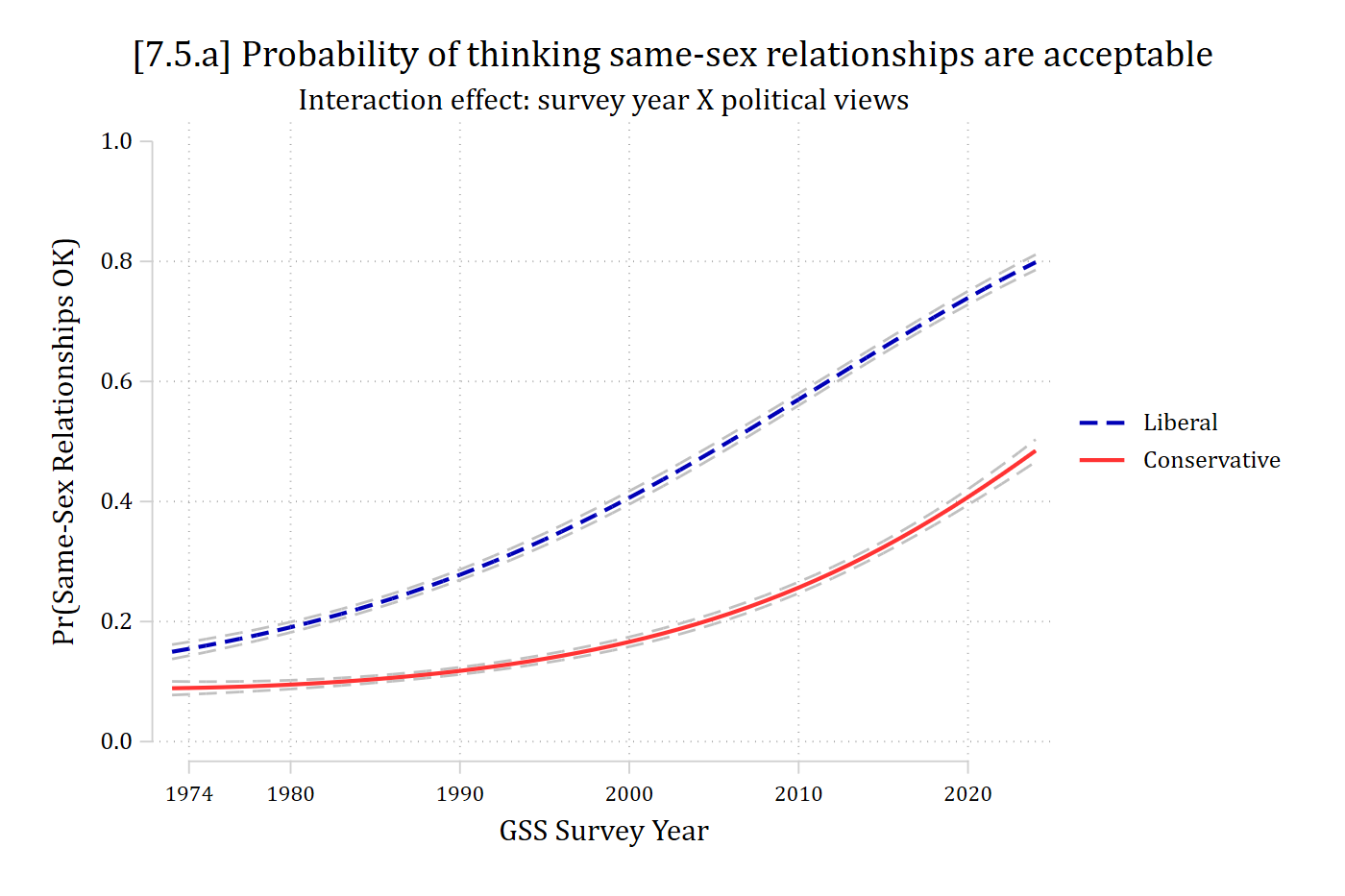
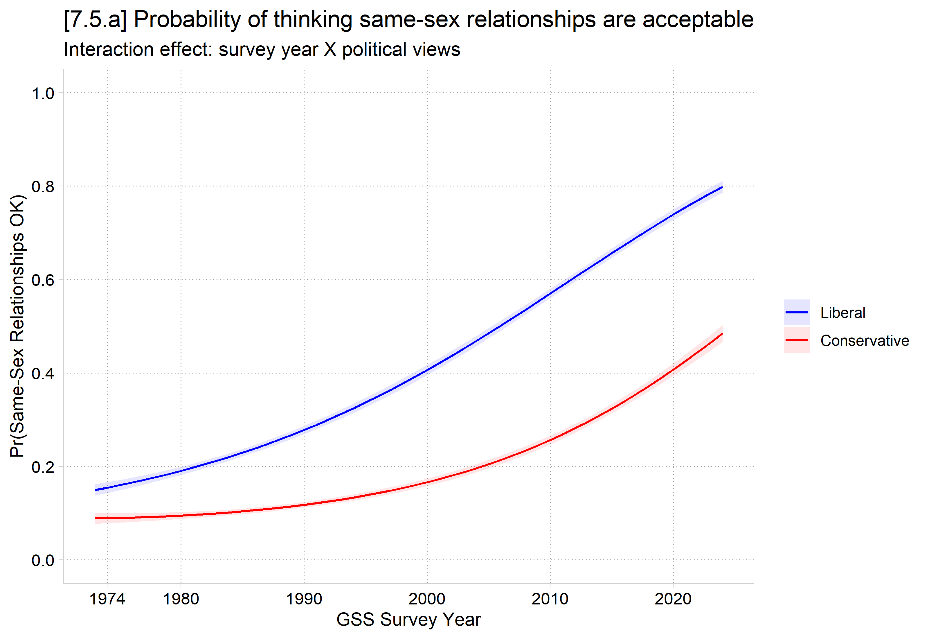
[7.5.a] Predicted probability of thinking same-sex relationships are acceptable by GSS survey year (1973 to 2024) for mainstream liberals (dashed blue) and mainstream conservatives (solid red). Both rise over time, slowly at first and then faster: liberals from about 0.15 to about 0.80, conservatives from about 0.09 to about 0.48, so the gap between them grows over time.

  • In R, use plot_predictions as normal, but specify only ideal typical values in the newdata statement
# Treat binary/nominal variables as factors
gss <- gss |>
  mutate(across(c(race3, woman, married, college), as_factor)) |>
  droplevels()

samemod <- glm(sameokB ~ poly(year1972, 2, raw = TRUE) * conviewSS + age + race3 +
  woman + faminc + married + college, data = gss, family = binomial(link = "logit"))

# 7.5.a - Plots of ideal types
plot_predictions(samemod, by = c("year1972", "conviewSS"),
  newdata = datagrid(year1972 = 1:52, conviewSS = c(2.5, 5.5), grid_type = "counterfactual")) +
  scale_color_manual(values = c("blue", "red"), labels = c("Liberal", "Conservative")) +
  scale_fill_manual(values = c("blue", "red"), labels = c("Liberal", "Conservative")) +
  scale_x_continuous(breaks = c(2, 8, 18, 28, 38, 48),
    labels = c(1974, 1980, 1990, 2000, 2010, 2020)) +
  scale_y_continuous(breaks = seq(0, 1, .2), limits = c(0, 1)) +
  labs(title = "[7.5.a] Probability of thinking same-sex relationships are acceptable",
    subtitle = "Interaction effect: survey year X political views",
    x = "GSS Survey Year", y = "Pr(Same-Sex Relationships OK)", color = NULL, fill = NULL)

[7.5.a] Predicted probability of thinking same-sex relationships are acceptable by GSS survey year (1973 to 2024) for mainstream liberals (dashed blue) and mainstream conservatives (solid red). Both rise over time, slowly at first and then faster: liberals from about 0.15 to about 0.80, conservatives from about 0.09 to about 0.48, so the gap between them grows over time.

In exploratory models, I found very strong evidence to prefer a model with year and year2 over a model with only year (∆BIC = 64)

Limitations of ideal type approach; tests of 2nd difference

  • “Although I find [the ideal type figure] a clear, intuitive, and helpful way to summarize these effects, it is also important to substantiate these intuitions with additional analyses and tests of statistical significance.” (Mize 2019 p.108-109)
  • The interaction effect is not directly tested in the ideal type figure
    • Always provide a statistical test for the interaction as well as the figure
  • If choosing substantive ideal types, test the ME of the focal IV across those values
    • 2nd difference is test of interaction
  • Absent theoretically informed values, I generally test the ME of the focal IV at:
    • The 5th (or 10th) percentile as a “low” ideal type*
    • The 50th percentile (median) as an “average” ideal type
    • The 95th (or 90th) percentile as a “high” ideal type*
      • And then all 2nd differences across these three ideal types

*I generally like 5th and 95th to represent truly low and high values; but with small samples or highly skewed distributions, I would use 10th and 90th percentiles

Tests of 2nd differences across ideal types

  • Using our two theoretical ideal types of “mainstream liberal” and “mainstream conservative”
// Tests of interaction (2nd diff) //
*Across theoretical ideal typical values
mecompare year1972, covariates(conviewSS=(2.5 5.5)) amount(sd) model(samemod)
Predicting: Pr(sameokB)
Marginal effects (N_samemod=37806)

                                 |  ME #   Estimate         SE      P>|z|
---------------------------------+---------------------------------------
year1972 + SD (centered)         |                                       
                   conviewSS=2.5 |     1      0.195      0.002      0.000
                   conviewSS=5.5 |     2      0.127      0.003      0.000
*2nd diff
metest 1 - 2
                                 |  estimate         se     pvalue 
---------------------------------+--------------------------------
 year1972_con~5 - year1972_con~5 |     0.067      0.004      0.000 
# Changes in continuous IVs centered on the observed values, like mecompare
options(marginaleffects_contrast_direction = "center")

# Tests of interaction (2nd diff)
# Across theoretical ideal typical values
mes <- avg_comparisons(samemod, variables = list(year1972 = sd(gss$year1972)),
  by = "conviewSS",
  newdata = datagrid(conviewSS = c(2.5, 5.5), grid_type = "counterfactual"))
mes

 conviewSS Estimate Std. Error    z Pr(>|z|)   S 2.5 % 97.5 %
       2.5    0.195    0.00225 86.5   <0.001 Inf 0.190  0.199
       5.5    0.127    0.00305 41.8   <0.001 Inf 0.121  0.133

Term: year1972
Type: response
Comparison: +15.9330355183697
# 2nd diff
hypotheses(mes, hypothesis = "b1 - b2 = 0")

 Hypothesis Estimate Std. Error    z Pr(>|z|)     S  2.5 % 97.5 %
    b1-b2=0   0.0675     0.0037 18.2   <0.001 243.9 0.0602 0.0748

Time has had a larger effect on mainstream liberals’ opinions of same-sex relationships than on mainstream conservatives’ opinions (2nd difference p < .001)

Tests of 2nd differences across empirical ideal types

*Across 5th, 50th, and 95th percentiles
sum conviewSS, d
                 Lib to Cons politics scale
-------------------------------------------------------------
      Percentiles      Smallest
 1%            1              1
 5%          1.5              1
10%            2              1       Obs              37,806
25%          2.5              1       Sum of wgt.      37,806

50%            4                      Mean           3.857853
                        Largest       Std. dev.       1.47418
75%            5              7
90%            6              7       Variance       2.173207
95%          6.5              7       Skewness       .1819076
99%            7              7       Kurtosis       2.191772
mecompare year1972, covariates(conviewSS=(1.5 4 6.5)) amount(sd) model(samemod
)
Predicting: Pr(sameokB)
Marginal effects (N_samemod=37806)

                                 |  ME #   Estimate         SE      P>|z|
---------------------------------+---------------------------------------
year1972 + SD (centered)         |                                       
                   conviewSS=1.5 |     1      0.206      0.003      0.000
                     conviewSS=4 |     2      0.167      0.002      0.000
                   conviewSS=6.5 |     3      0.099      0.004      0.000
*All 2nd diffs via the pwcompare option of metest
metest 1 2 3, pwcompare rowname("liberal" "moderate" "conservative")
                                 |  estimate         se     pvalue 
---------------------------------+--------------------------------
             moderate vs liberal |    -0.039      0.003      0.000 
         conservative vs liberal |    -0.107      0.006      0.000 
        conservative vs moderate |    -0.068      0.004      0.000 
# Across 5th, 50th, and 95th percentiles
quantile(gss$conviewSS, c(.05, .5, .95))
 5% 50% 95% 
1.5 4.0 6.5 
me <- avg_comparisons(samemod, variables = list(year1972 = sd(gss$year1972)),
  by = "conviewSS",
  newdata = datagrid(conviewSS = c(1.5, 4, 6.5), grid_type = "counterfactual"))
me

 conviewSS Estimate Std. Error    z Pr(>|z|)     S  2.5 % 97.5 %
       1.5   0.2061    0.00308 67.0   <0.001   Inf 0.2000  0.212
       4.0   0.1666    0.00198 84.2   <0.001   Inf 0.1627  0.170
       6.5   0.0987    0.00414 23.8   <0.001 414.4 0.0906  0.107

Term: year1972
Type: response
Comparison: +15.9330355183697
# All 2nd diffs
hypotheses(me, hypothesis = ~ pairwise)

  Hypothesis Estimate Std. Error     z Pr(>|z|)     S   2.5 %  97.5 %
 (b2) - (b1)  -0.0395    0.00303 -13.0   <0.001 126.5 -0.0454 -0.0335
 (b3) - (b1)  -0.1073    0.00574 -18.7   <0.001 257.2 -0.1186 -0.0961
 (b3) - (b2)  -0.0679    0.00361 -18.8   <0.001 260.1 -0.0749 -0.0608

Effect of year at 5th, 50th, and 95th percentiles of political views; and all 2nd differences

Published example

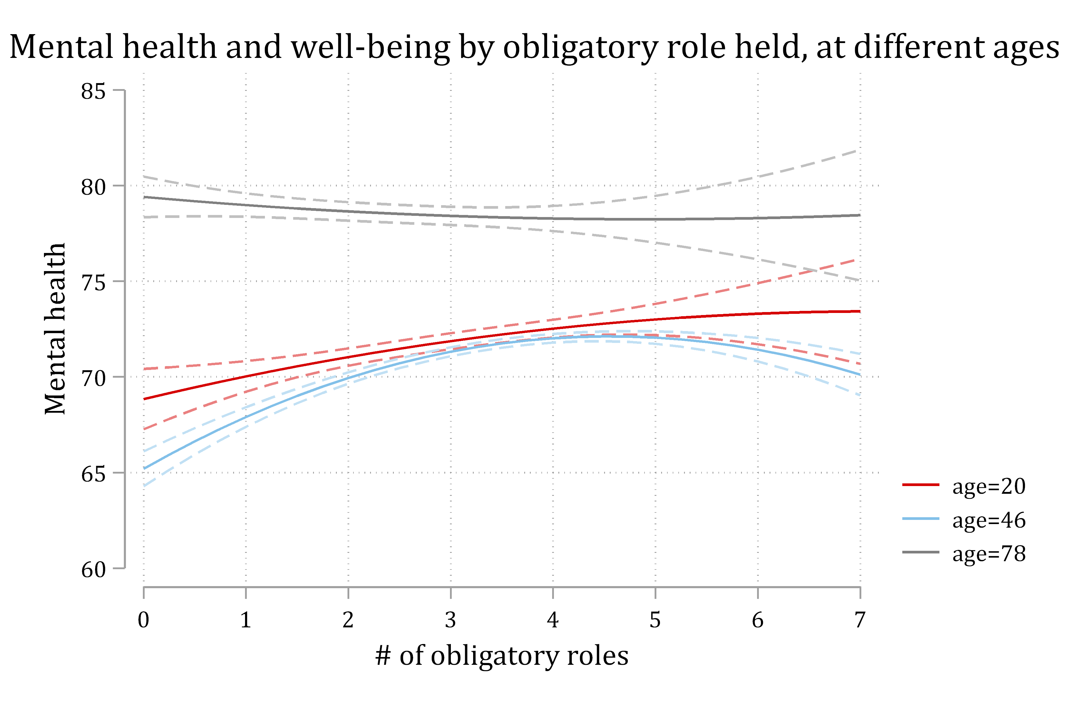
Figure from Mize and Kincaid (2025): mental health and well-being by number of obligatory roles held (0 to 7), at ages 20, 46, and 78, with confidence intervals. At age 20, mental health rises with more roles; at age 46 it rises and then flattens; at age 78 it is nearly flat or declines slightly.

*Ex from Mize and Kincaid 2025

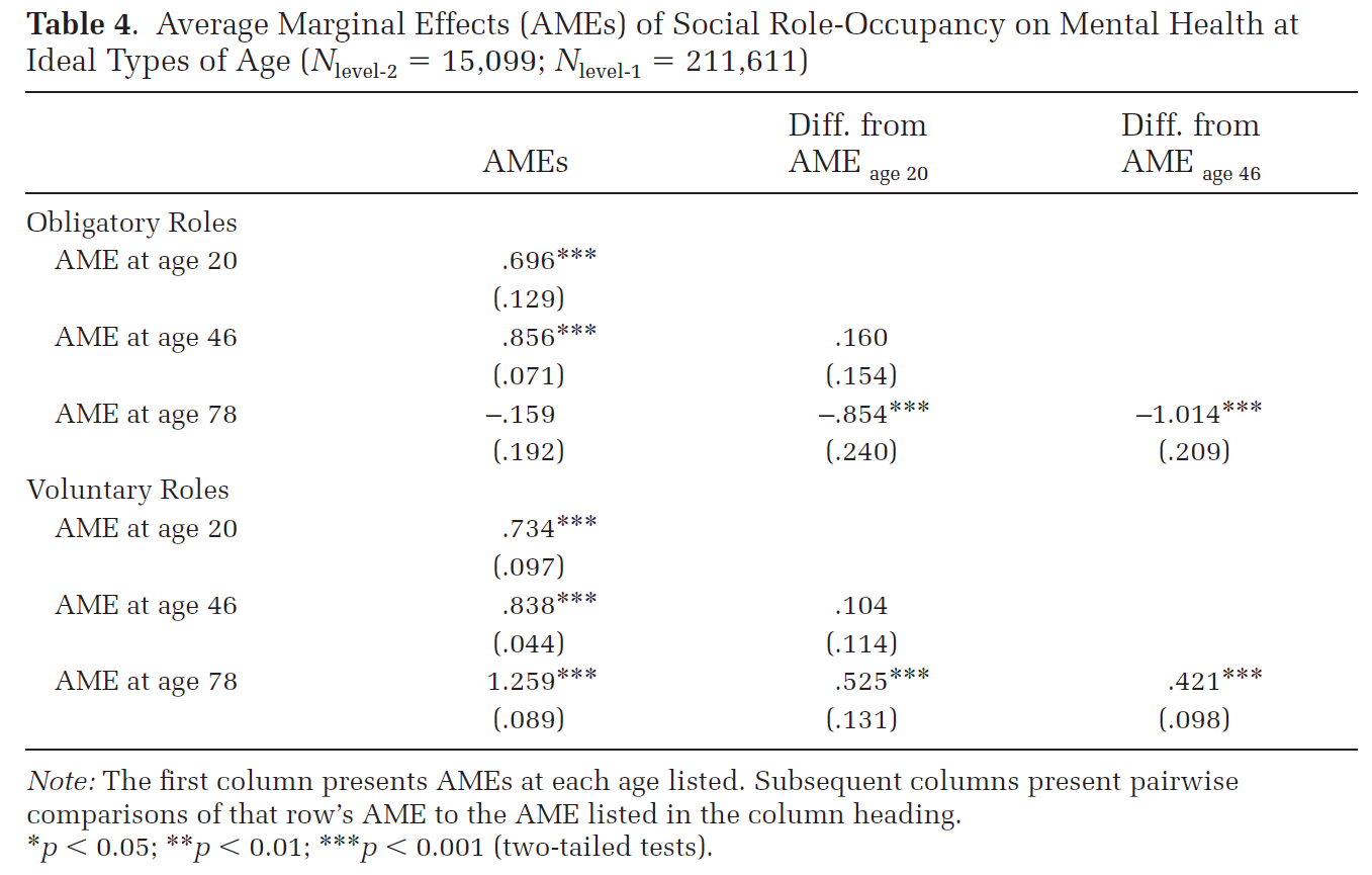
Table 4 from Mize and Kincaid (2025): average marginal effects of social role-occupancy on mental health at ideal types of age (20, 46, and 78), for obligatory and voluntary roles, with columns for the AMEs and for differences from the AME at age 20 and at age 46. For example, the obligatory-role AME is .696 at age 20, .856 at age 46, and -.159 at age 78.

*Ex from Mize and Kincaid 2025

Marginal effects plots

  • Marginal effects plots are an effective way to present a more direct test of the interaction
  • Plot the ME of one continuous IV across the range of the other IV
    • A flat line suggests no interaction: size of ME of focal IV is similar across range of moderating IV
    • Non-flat lines suggest interaction: size of ME of focal IV differs across range
  • Can make two plots; one for each IV’s ME
    • But, sometimes strong theory to just show ME of focal IV across (trimmed) range of moderating IV

Marginal effects plots in Stata and R

  • In Stata, calculate ME of focal continuous IV using margins, dydx( ) for the instantaneous rate of change; or mecompare with the store() option for a discrete change (e.g. +1, +SD)
    • Plot with marginsplot or coefplot
margins, dydx(conviewSS) at(year1972=(1(1)52))

marginsplot, yline(0) …
//#7.5.b & 7.5.c - Plots of marginal effects of one var across range of other 
//
**7.5.b Marginal effect of Political Views across range of year
*mecompare can be used for discrete change ME (e.g. +1 or +SD)
qui mecompare conviewSS, models(samemod) covariates(year1972=(1(1)52)) amount(
sd) store(pv)
coefplot pv_samemod, vertical recast(connected) color(black) lwid(*1.5) msym(n
one) ///
    ciopts(recast(rline) lpattern(dash) color(gs12)) yline(0) ///
    ylabel(-0.25(0.05)0.05) xtitle("GSS survey year") ///
    xlabel(2 "1974" 8 "1980" 18 "1990" 28 "2000" 38 "2010" 48 "2020", labsize(
2.5)) ///
    ytitle("AME of +SD cons. political views") ///
    title("[7.5.b] AME of political views (lib to cons.) by survey year") ///
    note("Negative effects indicate conservatives are less supportive of same-
sex relationships")

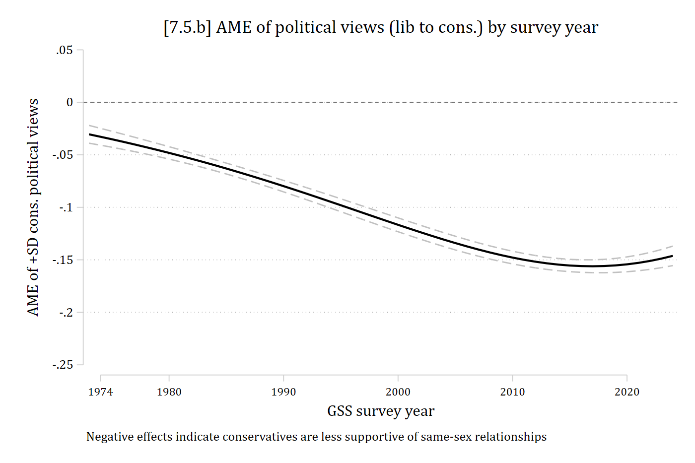
[7.5.b] Average marginal effect of a standard deviation increase in conservative political views on the probability of thinking same-sex relationships are acceptable, by GSS survey year, with confidence intervals and a line at zero. The effect is negative in every year and grows stronger over time, from about -0.03 in 1973 to about -0.15 by the late 2010s, then levels off.

# 7.5.b Marginal effect of Political Views across range of year
plot_comparisons(samemod, variables = list(conviewSS = sd(gss$conviewSS)),
  by = "year1972",
  newdata = datagrid(year1972 = 1:52, grid_type = "counterfactual")) +
  geom_hline(yintercept = 0, linetype = "dashed") +
  scale_x_continuous(breaks = c(2, 8, 18, 28, 38, 48),
    labels = c(1974, 1980, 1990, 2000, 2010, 2020)) +
  scale_y_continuous(breaks = seq(-.25, .05, .05), limits = c(-.25, .05)) +
  labs(title = "[7.5.b] AME of political views (lib to cons.) by survey year",
    caption = "Negative effects indicate conservatives are less supportive of same-sex relationships",
    x = "GSS survey year", y = "AME of +SD cons. political views")

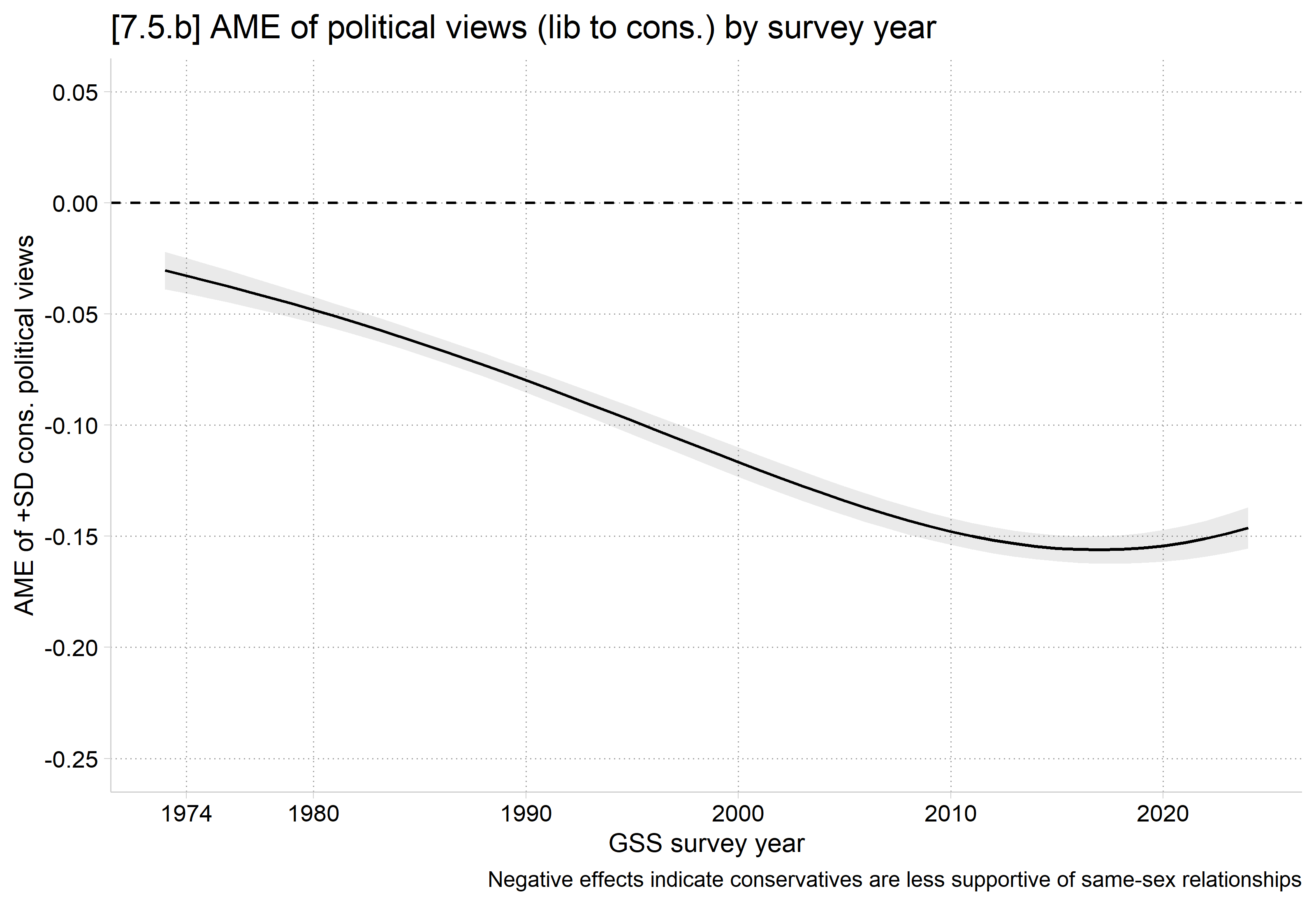
[7.5.b] Average marginal effect of a standard deviation increase in conservative political views on the probability of thinking same-sex relationships are acceptable, by GSS survey year, with confidence intervals and a line at zero. The effect is negative in every year and grows stronger over time, from about -0.03 in 1973 to about -0.15 by the late 2010s, then levels off.

Always include a line at zero indicating a null effect

**7.5.c - Marginal effect of Year (time) across range of political views //
*mecompare can be used for discrete change ME (e.g. +1 or +SD)
qui mecompare year1972, models(samemod) covariates(conviewSS=(1(.5)7)) amount(
sd) store(mes)
coefplot mes_samemod, vertical recast(connected) color(purple) lwid(*1.5) msym
(none) ///
    ciopts(recast(rline) lpattern(dash) color(purple*.5)) yline(0) ///
    ylabel(-0.05(0.05)0.25) xtitle("Political views") ///
    xlabel(1 `""1" "Most liberal""' 3 "2" 5 "3" 7 `""4" "Middle""' ///
        9 "5" 11 "6" 13 `""7" "Most conservative""', labsize(2.5)) ///
    ytitle("AME of +SD elapsed years") ///
    title("[7.5.c] AME of survey year (passage of time) by political views") /
//
    note("Positive effects = group has become more supportive of same-sex rela
tionships over time")

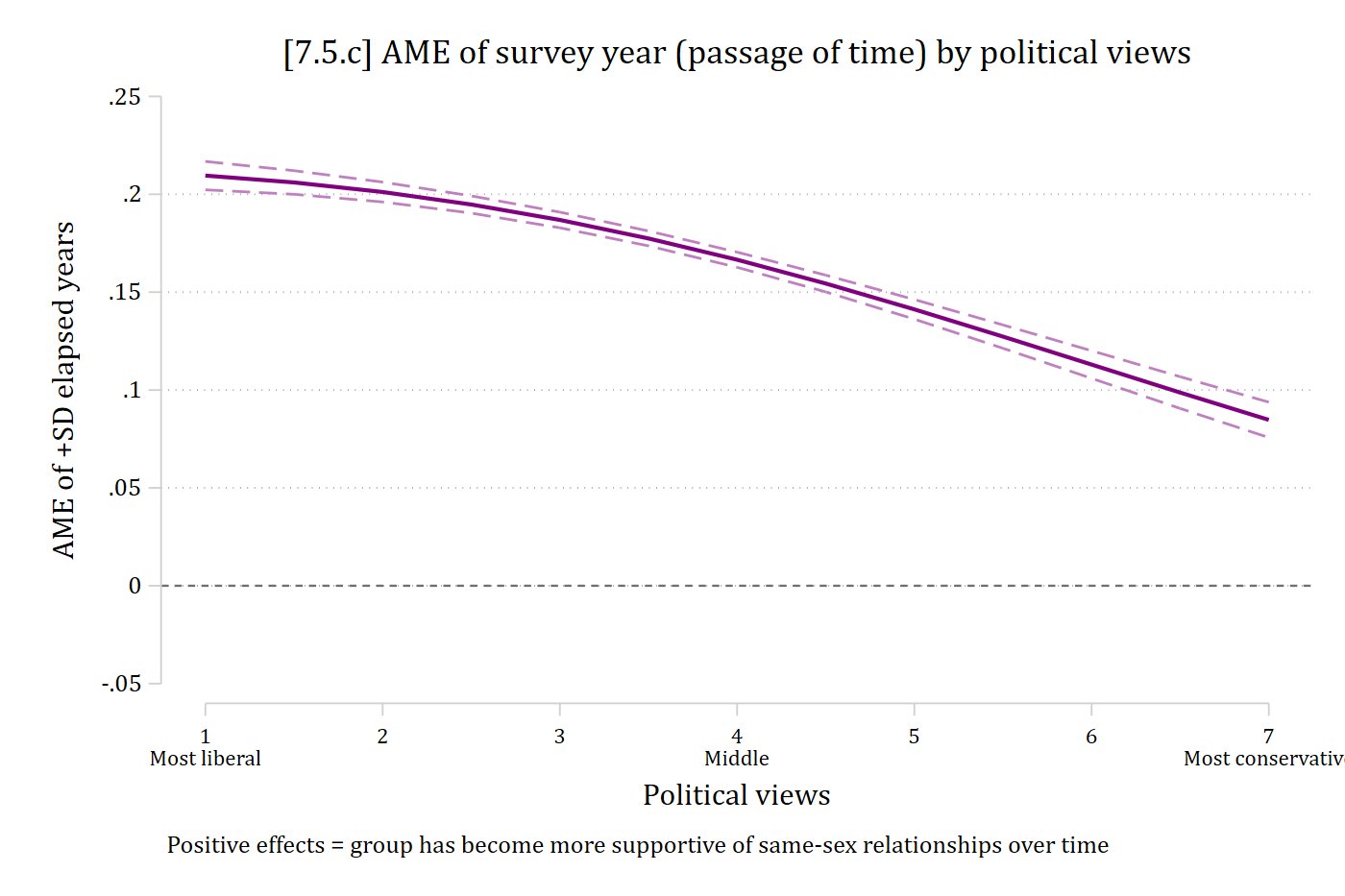
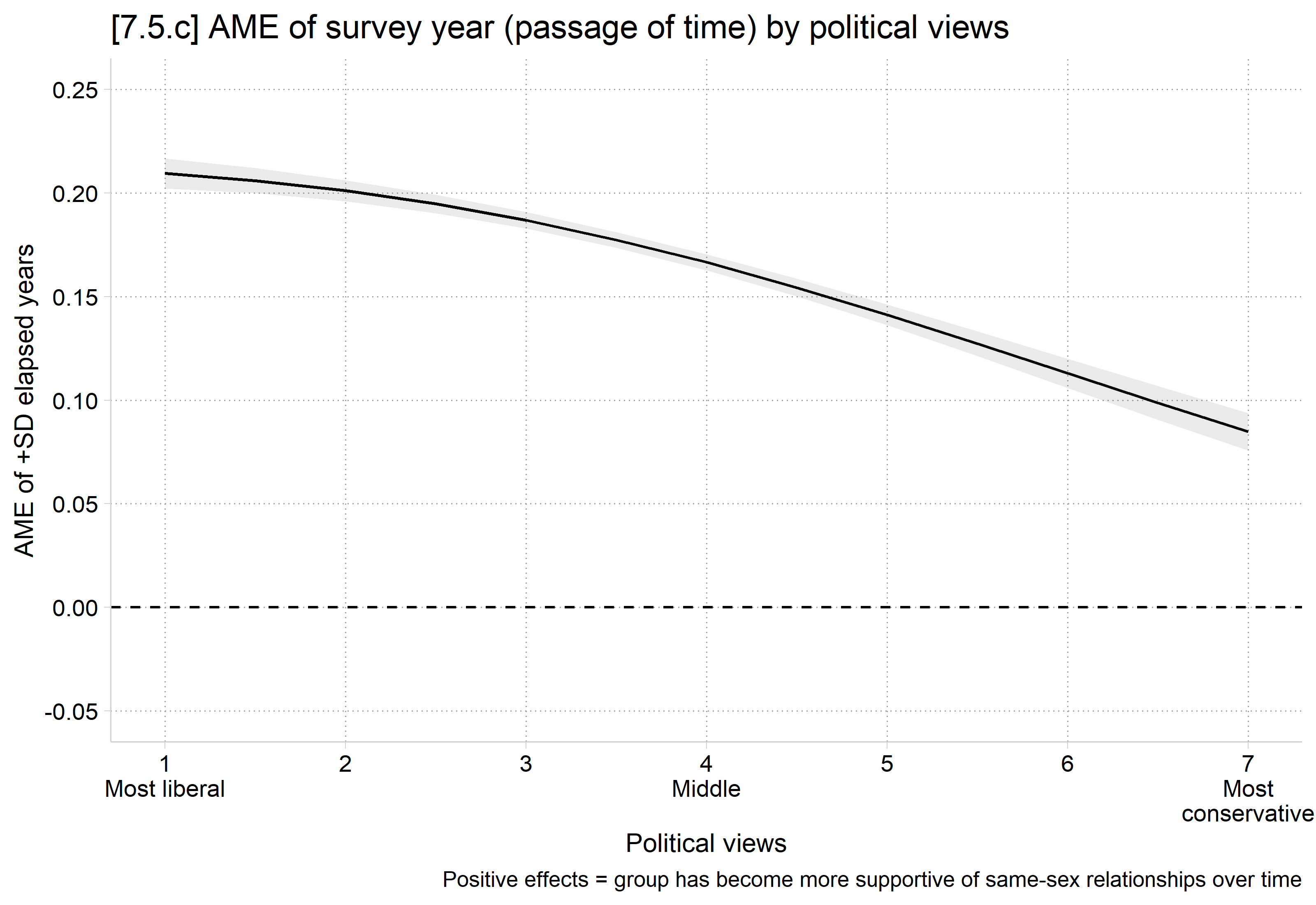
[7.5.c] Average marginal effect of a standard deviation increase in survey year (the passage of time) on the probability of thinking same-sex relationships are acceptable, across political views from most liberal (1) to most conservative (7), with confidence intervals and a line at zero. The effect is positive everywhere and declines steadily from about 0.21 for the most liberal to about 0.09 for the most conservative.

# 7.5.c - Marginal effect of Year (time) across range of political views
plot_comparisons(samemod, variables = list(year1972 = sd(gss$year1972)),
  by = "conviewSS",
  newdata = datagrid(conviewSS = seq(1, 7, .5), grid_type = "counterfactual")) +
  geom_hline(yintercept = 0, linetype = "dashed") +
  scale_x_continuous(breaks = 1:7, labels = c("1\nMost liberal", "2", "3", "4\nMiddle",
    "5", "6", "7\nMost\nconservative")) +
  scale_y_continuous(breaks = seq(-.05, .25, .05), limits = c(-.05, .25)) +
  labs(title = "[7.5.c] AME of survey year (passage of time) by political views",
    caption = "Positive effects = group has become more supportive of same-sex relationships over time",
    x = "Political views", y = "AME of +SD elapsed years")

[7.5.c] Average marginal effect of a standard deviation increase in survey year (the passage of time) on the probability of thinking same-sex relationships are acceptable, across political views from most liberal (1) to most conservative (7), with confidence intervals and a line at zero. The effect is positive everywhere and declines steadily from about 0.21 for the most liberal to about 0.09 for the most conservative.

Second difference tests

  • The recommended tests of second differences are the same regardless as to whether you use an ideal types or marginal effects plot
    • Tests above at ideal typical values of moderator, or at 5th, 50th, and 95th percentile of moderating IV are appropriate
  • Here, flipping the focal and moderating IVs, just for illustration
// Ex 2nd difference flipping focal and moderating IV //
mecompare conviewSS, models(samemod) covariates(year1972=(1 52)) amount(sd)
Predicting: Pr(sameokB)
Marginal effects (N_samemod=37806)

                                 |  ME #   Estimate         SE      P>|z|
---------------------------------+---------------------------------------
conviewSS + SD (centered)        |                                       
                      year1972=1 |     1     -0.030      0.004      0.000
                     year1972=52 |     2     -0.146      0.005      0.000
# Ex 2nd difference flipping focal and moderating IV
me <- avg_comparisons(samemod, variables = list(conviewSS = sd(gss$conviewSS)),
  by = "year1972",
  newdata = datagrid(year1972 = c(1, 52), grid_type = "counterfactual"))
me

 year1972 Estimate Std. Error      z Pr(>|z|)     S   2.5 % 97.5 %
        1  -0.0304    0.00432  -7.04   <0.001  38.9 -0.0389 -0.022
       52  -0.1462    0.00473 -30.91   <0.001 694.4 -0.1555 -0.137

Term: conviewSS
Type: response
Comparison: +1.47418022536454

Example write-up

metest 2 - 1
                                 |  estimate         se     pvalue 
---------------------------------+--------------------------------
 conviewSS_y~52 - conviewSS_ye~1 |    -0.116      0.006      0.000 
hypotheses(me, hypothesis = "b2 - b1 = 0")

 Hypothesis Estimate Std. Error     z Pr(>|z|)     S  2.5 % 97.5 %
    b2-b1=0   -0.116    0.00558 -20.7   <0.001 314.8 -0.127 -0.105

Figure # illustrates that conservative political views are consistently associated with less support for same-sex relationships, across all years of the GSS. But there is variation over time: the effect of political views in more recent years is much stronger than the effect of political views in the earliest surveys in the 1970s. For illustration, consider the earliest and latest year in the GSS: in 1973 a standard deviation increase in conservatism predicted only a 3 percentage point decline in support for same-sex relationships; that same +SD change in 2024 predicts a 15 percentage point decline (2nd difference = -0.116, p < .001).

Contour plots

  • One of the primary difficulties of interpreting continuous X continuous interactions is thinking in two dimensions
  • Contour plots present the Pr(y = 1) at the intersection of the two continuous variables included in the interaction
    • Each IV makes up an axis (one on x; one on y)
    • Color is used to present the information on the Pr(y = 1)
  • These work best when you can use color so you can easily distinguish the different Pr(y = 1)
    • So, works well in a talk or a journal that allows color

*These plots are made in a different way in Stata than other plots I’ve shown. See Appendix A7.5 for the full details

Contour plots in Stata and R

  • In Stata, use margins to make predictions at all combinations across the (trimmed) ranges of both continuous IVs
    • Make the plot* using twoway contour
      • Syntax: (1) variable with the predictions comes first, (2) followed by the IV you want on the x-axis, then (3) the IV you want on the y-axis

*See Appendix A7.5 for the full Stata details

//#7.5.d - 7.5.h: Contour plots //
est restore samemod
(results samemod are active now)
*Make predictions at all combinations of both continuous IVs
qui margins, at(conviewSS=(1(.5)7) year1972=(1(1)52)) ///
    saving(preds, replace)
*Load dataset of predictions; rename vars to be plotted
use preds, clear
(Created by command margins; also see char list)
rename _at1 year1972
rename _at2 conviewSS
rename _margin pr_sameok
*7.5.g - Ordinal color scheme viridis; colorpalette saves the colors in r(p)
colorpalette viridis, n(22) reverse nograph
twoway (contour pr_sameok conviewSS year1972, levels(20) ccolors(`r(p)')), ///
    xlabel(2 "1974" 8 "1980" 18 "1990" 28 "2000" 38 "2010" 48 "2020", labsize(
2.5) nogrid) ///
    ylabel(1 `""Very" "liberal""' 2.5 "Liberal" 4 "Middle" ///
        5.5 "Conservative" 7 `""Very" "conservative""', nogrid) ///
    zlabel(0(0.1)1, format(%2.1f)) ztitle("Pr(Same-Sex Relationships OK)") ///
    xtitle("") ytitle("") ysize(4) xsize(6) ///
    title("[7.5.g] Predicted probability of thinking same-sex relationships ar
e acceptable") ///
    subtitle("Interaction: Political beliefs X survey year")

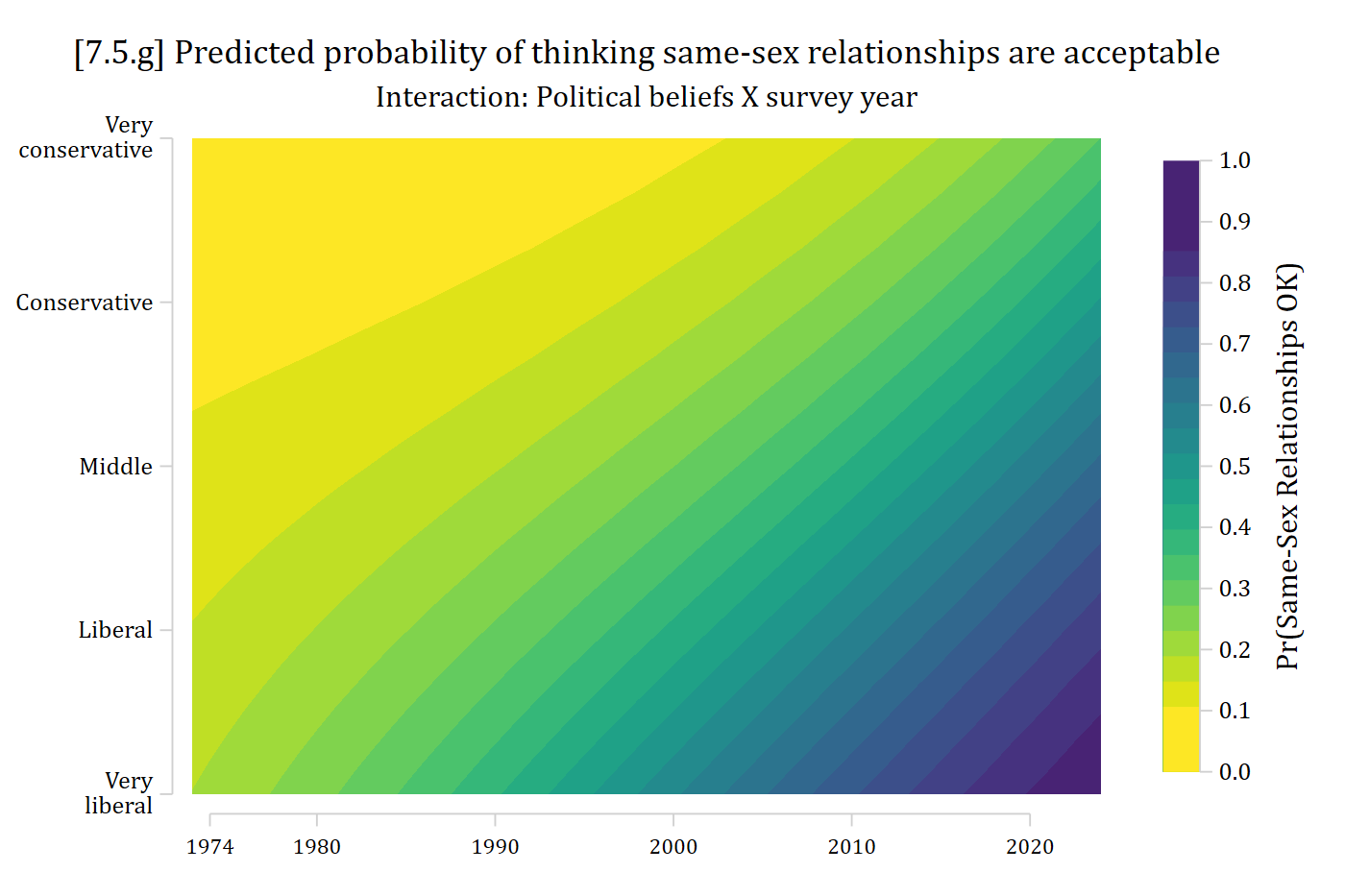
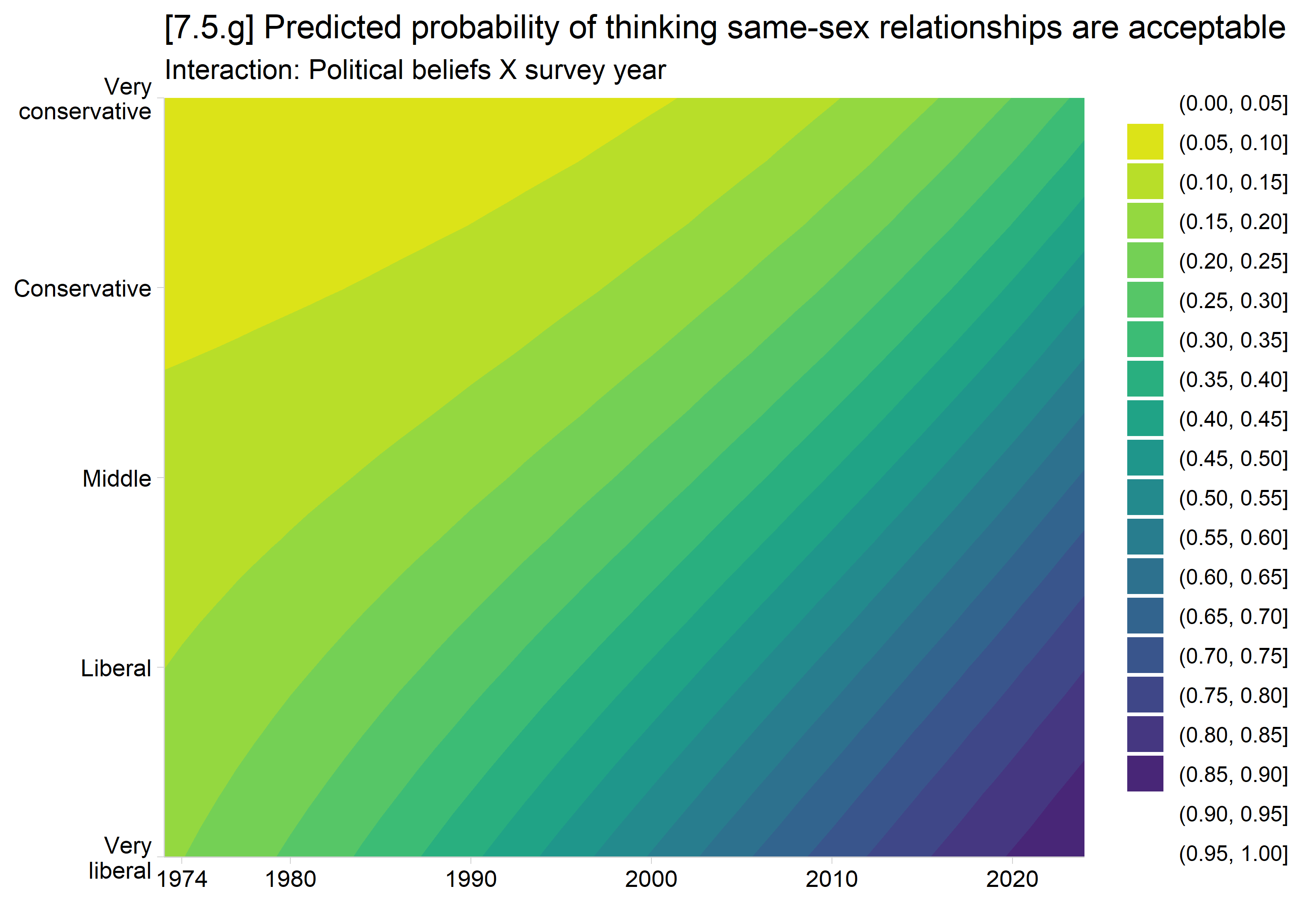
[7.5.g] Contour plot in the viridis colors of the predicted probability of thinking same-sex relationships are acceptable, with survey year (1973 to 2024) on the x-axis and political views (very liberal to very conservative) on the y-axis. Probabilities are lowest (about 0.07, yellow) for conservatives in the 1970s and highest (about 0.9, dark purple) for liberals in the most recent years; the bands slant so that liberals reach each level of support years before conservatives do.

  • In R, save predictions for all combinations of the continuous IVs
    • Use ggplot and geom_contour_filled
      • Syntax: (1) IV you want on the x-axis, (2) the IV you want on the y-axis, then (3) z dimension is the saved estimate of Pr(y=1)
# 7.5.d - 7.5.h: Contour plots
# Make predictions at all combinations of both continuous IVs (one year at a time,
# which needs much less memory than one call for all 676 combinations)
pr4 <- bind_rows(lapply(1:52, function(y) {
  avg_predictions(samemod, by = c("conviewSS", "year1972"), vcov = FALSE,
    newdata = datagrid(conviewSS = seq(1, 7, .5), year1972 = y,
      grid_type = "counterfactual"))
}))

# 7.5.g - Ordinal color scheme viridis (the default)
ggplot(pr4, aes(x = year1972, y = conviewSS, z = estimate)) +
  geom_contour_filled(breaks = seq(0, 1, .05)) +
  scale_fill_viridis_d(direction = -1, drop = FALSE) +
  scale_x_continuous(breaks = c(2, 8, 18, 28, 38, 48),
    labels = c(1974, 1980, 1990, 2000, 2010, 2020), expand = c(0, 0)) +
  scale_y_continuous(breaks = c(1, 2.5, 4, 5.5, 7), labels = c("Very\nliberal",
    "Liberal", "Middle", "Conservative", "Very\nconservative"), expand = c(0, 0)) +
  labs(title = "[7.5.g] Predicted probability of thinking same-sex relationships are acceptable",
    subtitle = "Interaction: Political beliefs X survey year",
    x = NULL, y = NULL, fill = "Pr(Same-Sex\nRelationships OK)")

[7.5.g] Contour plot in the viridis colors of the predicted probability of thinking same-sex relationships are acceptable, with survey year (1973 to 2024) on the x-axis and political views (very liberal to very conservative) on the y-axis. Probabilities are lowest (about 0.07, yellow) for conservatives in the 1970s and highest (about 0.9, dark purple) for liberals in the most recent years; the bands slant so that liberals reach each level of support years before conservatives do.

*7.5.d - Rainbow colors version -- accomplished with starting color scolor(red
)
*   ending color ecolor(purple) and crule(hue)
twoway (contour pr_sameok conviewSS year1972, levels(20) ///
    scolor(red) ecolor(purple) crule(hue)), ///
    xlabel(2 "1974" 8 "1980" 18 "1990" 28 "2000" 38 "2010" 48 "2020", labsize(
2.5) nogrid) ///
    ylabel(1 `""Very" "liberal""' 2.5 "Liberal" 4 "Middle" ///
        5.5 "Conservative" 7 `""Very" "conservative""', nogrid) ///
    zlabel(0(0.1)1, format(%2.1f)) ztitle("Pr(Same-Sex Relationships OK)") ///
    xtitle("") ytitle("") ysize(4) xsize(6) ///
    title("[7.5.d] Predicted probability of thinking same-sex relationships ar
e acceptable") ///
    subtitle("Interaction: Political beliefs X survey year")

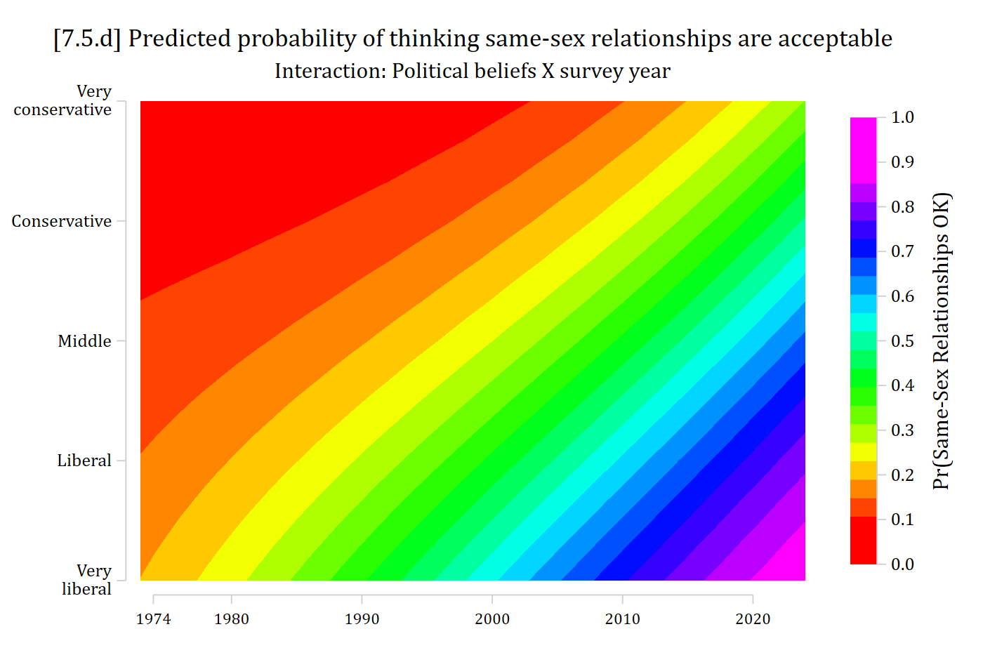
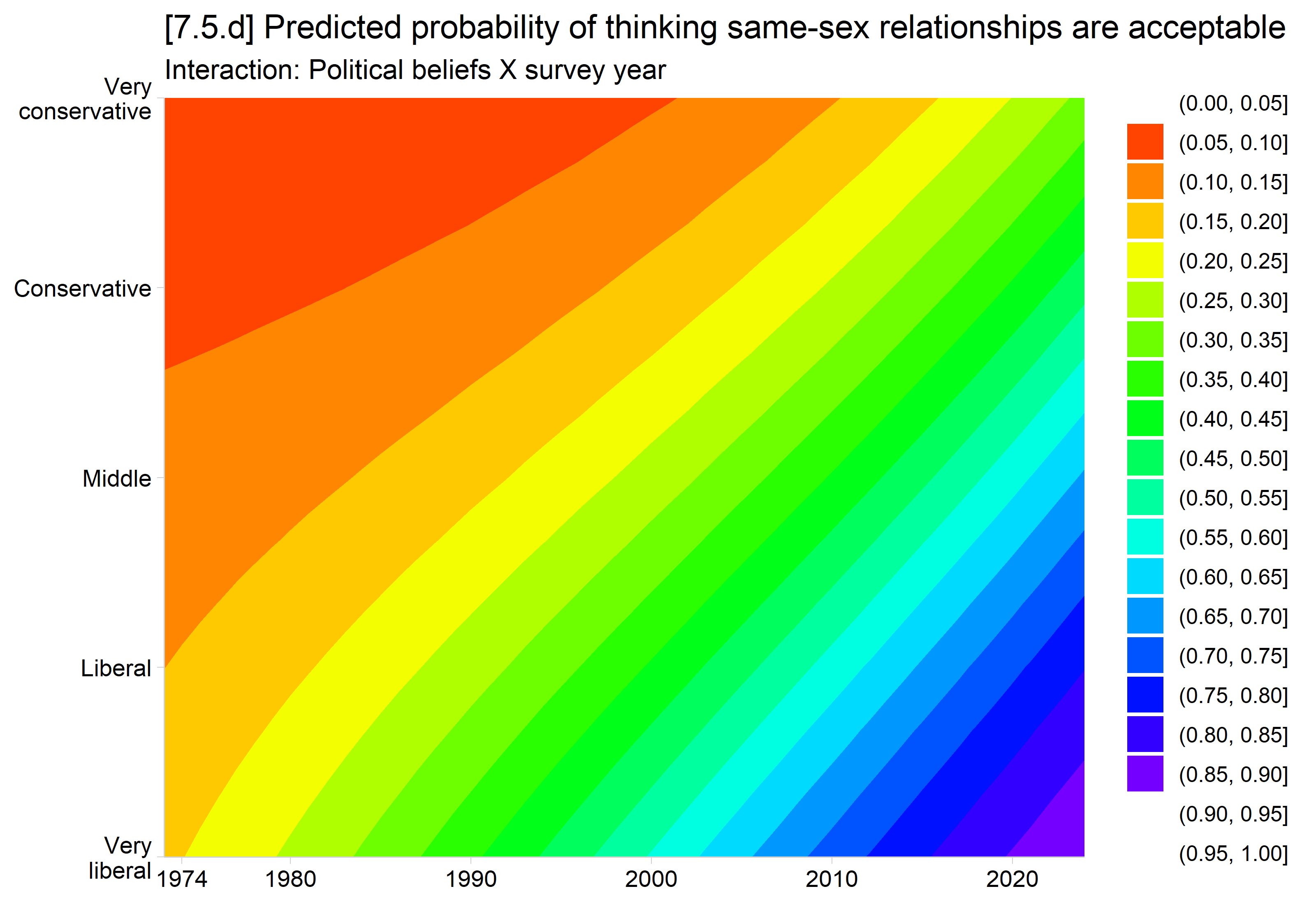
[7.5.d] The same contour plot in rainbow colors, from red (lowest probabilities, conservatives in the 1970s) through orange, yellow, green, and blue to purple (highest probabilities, liberals in recent years), with survey year on the x-axis and political views on the y-axis.

# 7.5.d - Rainbow colors version
ggplot(pr4, aes(x = year1972, y = conviewSS, z = estimate)) +
  geom_contour_filled(breaks = seq(0, 1, .05)) +
  scale_fill_manual(values = rainbow(20, end = .83), drop = FALSE) +
  scale_x_continuous(breaks = c(2, 8, 18, 28, 38, 48),
    labels = c(1974, 1980, 1990, 2000, 2010, 2020), expand = c(0, 0)) +
  scale_y_continuous(breaks = c(1, 2.5, 4, 5.5, 7), labels = c("Very\nliberal",
    "Liberal", "Middle", "Conservative", "Very\nconservative"), expand = c(0, 0)) +
  labs(title = "[7.5.d] Predicted probability of thinking same-sex relationships are acceptable",
    subtitle = "Interaction: Political beliefs X survey year",
    x = NULL, y = NULL, fill = "Pr(Same-Sex\nRelationships OK)")
[7.5.d] The same contour plot in rainbow colors, from red (lowest probabilities, conservatives in the 1970s) through orange, yellow, green, and blue to purple (highest probabilities, liberals in recent years), with survey year on the x-axis and political views on the y-axis.

*7.5.e - A continuous rainbow color version accomplished by starting color sco
lor(red),
*   ending color ecolor(purple), crule(hue), and specifying levels(#) instead
*   of ccuts(). Note max levels is 500
twoway (contour pr_sameok conviewSS year1972, levels(500) ///
    scolor(red) ecolor(purple) crule(hue)), ///
    xlabel(2 "1974" 8 "1980" 18 "1990" 28 "2000" 38 "2010" 48 "2020", labsize(
2.5) nogrid) ///
    ylabel(1 `""Very" "liberal""' 2.5 "Liberal" 4 "Middle" ///
        5.5 "Conservative" 7 `""Very" "conservative""', nogrid) ///
    zlabel(0(0.1)1, format(%2.1f)) ztitle("Pr(Same-Sex Relationships OK)") ///
    xtitle("") ytitle("") ysize(4) xsize(6) ///
    title("[7.5.e] Predicted probability of thinking same-sex relationships ar
e acceptable") ///
    subtitle("Interaction: Political beliefs X survey year")

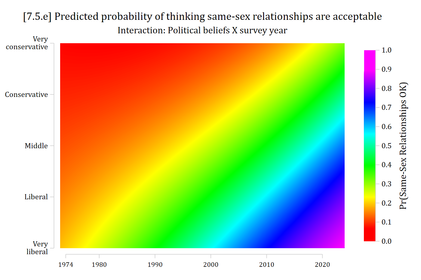
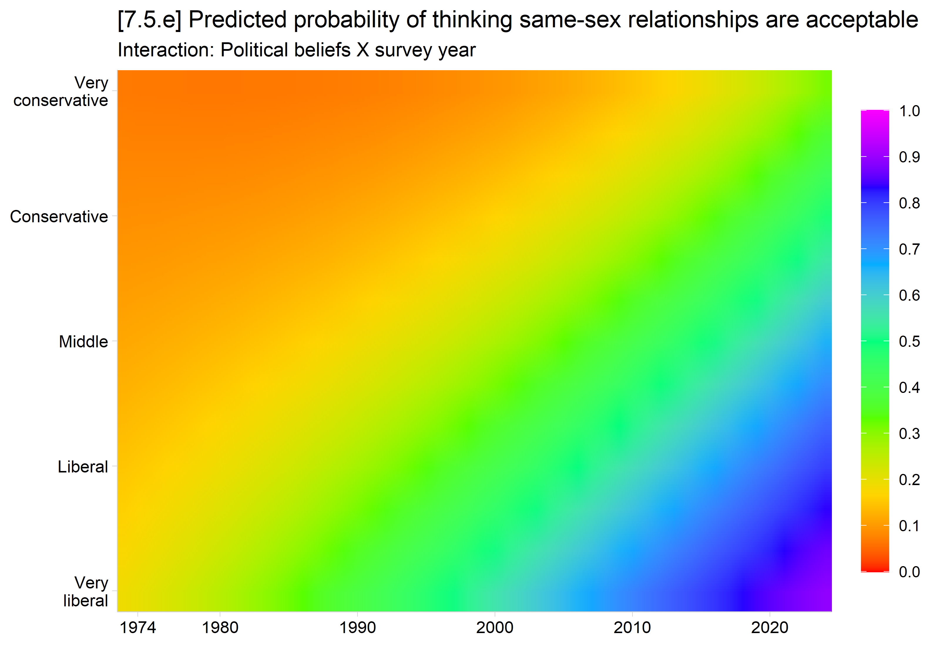
[7.5.e] The same contour plot with a smooth, continuous rainbow color gradient (500 levels) instead of distinct bands, from red for the lowest probabilities to purple for the highest.

# 7.5.e - A continuous rainbow color version
ggplot(pr4, aes(x = year1972, y = conviewSS, fill = estimate)) +
  geom_raster(interpolate = TRUE) +
  scale_fill_gradientn(colors = rainbow(7, end = .83), limits = c(0, 1),
    breaks = seq(0, 1, .1)) +
  scale_x_continuous(breaks = c(2, 8, 18, 28, 38, 48),
    labels = c(1974, 1980, 1990, 2000, 2010, 2020), expand = c(0, 0)) +
  scale_y_continuous(breaks = c(1, 2.5, 4, 5.5, 7), labels = c("Very\nliberal",
    "Liberal", "Middle", "Conservative", "Very\nconservative"), expand = c(0, 0)) +
  labs(title = "[7.5.e] Predicted probability of thinking same-sex relationships are acceptable",
    subtitle = "Interaction: Political beliefs X survey year",
    x = NULL, y = NULL, fill = "Pr(Same-Sex\nRelationships OK)") +
  theme(legend.key.height = unit(2, "cm"))

[7.5.e] The same contour plot with a smooth, continuous rainbow color gradient (500 levels) instead of distinct bands, from red for the lowest probabilities to purple for the highest.

Back to top