5.4 Parallel Regression Assumption

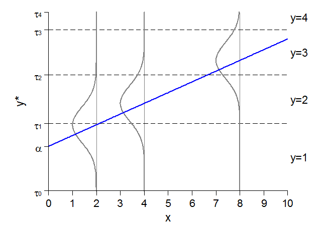
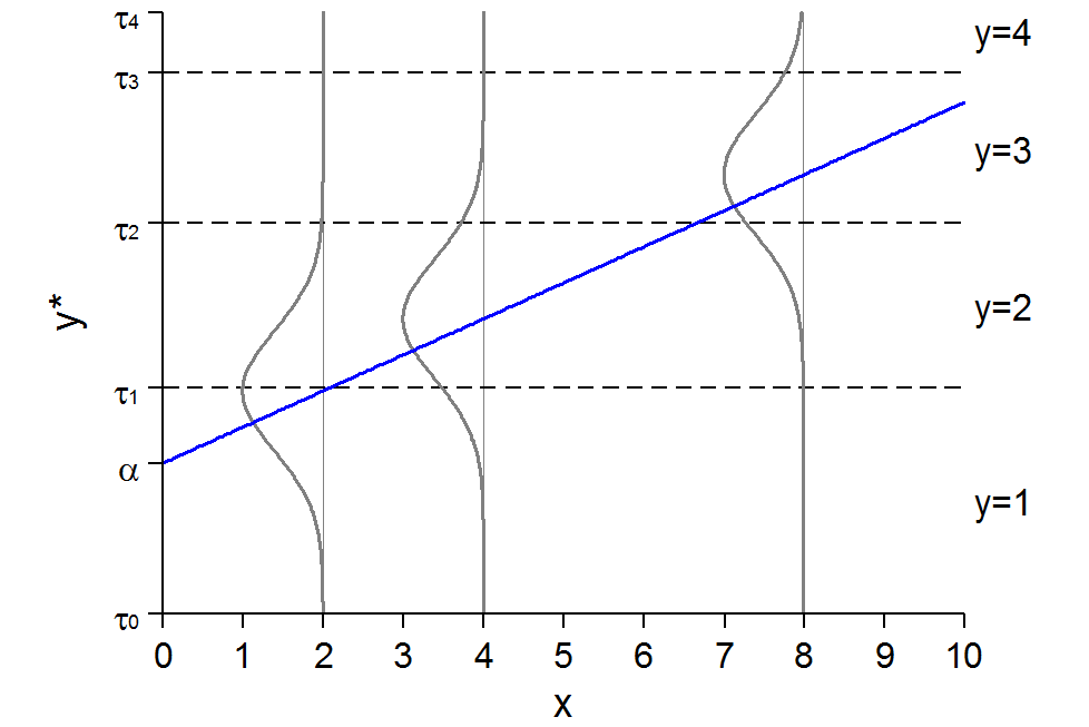
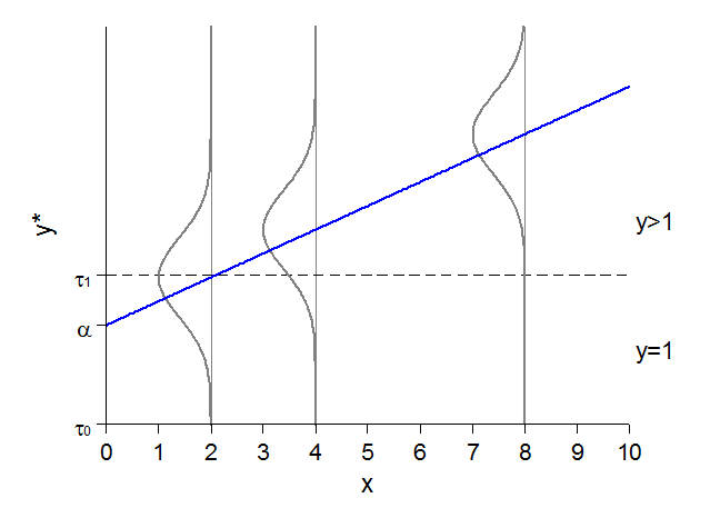
Latent y-star rising linearly with x, with normal error distributions drawn at x = 2, 4, and 8; dashed lines at the thresholds tau 1, tau 2, and tau 3 split each distribution into the probabilities of y = 1 to y = 4.

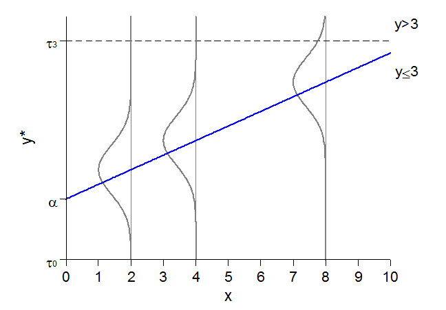
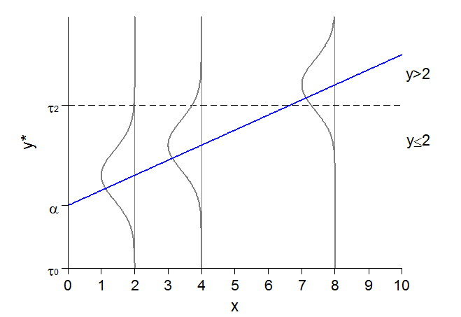
Dichotomizing at different τ’s does not change the slope

The same latent regression line dichotomized at tau 1 into y = 1 and y > 1.

The same latent regression line dichotomized at tau 3 into y ≤ 3 and y > 3.

The same latent regression line dichotomized at tau 2 into y ≤ 2 and y > 2.

The latent regression line with all three thresholds, splitting y into categories 1 to 4.

Ordinal logit as a set of parallel binary regressions

  • The assumption of equal slopes in the ordinal model is interchangeably called:

    • Proportional odds assumption
    • Parallel regression assumption
  • Suppose y has 4 outcomes (e.g. SD, D, A, SA)

  • Create 4 - 1 = 3 binary variables

    B1=1 if y ≤ 1, else 0

    B2=1 if y ≤ 2, else 0

    B3=1 if y ≤ 3, else 0

  • Fit three binary logits where both intercepts (α) and coefficients (β) can vary across each model:

\[\begin{aligned} \Pr(B_{1}) &= \Pr(y \leq 1) = F(\alpha_{1} + \beta_{1,1}x_{1} + \beta_{2,1}x_{2}) \\ \Pr(B_{2}) &= \Pr(y \leq 2) = F(\alpha_{2} + \beta_{1,2}x_{1} + \beta_{2,2}x_{2}) \\ \Pr(B_{3}) &= \Pr(y \leq 3) = F(\alpha_{3} + \beta_{1,3}x_{1} + \beta_{2,3}x_{2}) \end{aligned}\]

  • Ordinal logit simultaneously fits the equations:

\[\begin{aligned} \Pr(y \leq 1) &= F(\alpha_{1} + \beta_{1}x_{1} + \beta_{2}x_{2}) \\ \Pr(y \leq 2) &= F(\alpha_{2} + \beta_{1}x_{1} + \beta_{2}x_{2}) \\ \Pr(y \leq 3) &= F(\alpha_{3} + \beta_{1}x_{1} + \beta_{2}x_{2}) \end{aligned}\]

  • The β’s are constrained to be identical in all equations
  • The intercepts (α) vary by cumulative outcome (these are the estimates of the thresholds \(\tau\))

With and without the parallel regression assumption

*Simulate data to show parallel regression assumption
clear
set seed 30004
set obs 2000
Number of observations (_N) was 0, now 2,000.
matrix P = (1, 0.2 \ 0.2, 1) // Small correlation
corr2data x1 x2, n(2000) cov(P)
gen c = rnormal(0,10)
gen b = c
replace b = 0 in 1/1000
(1,000 real changes made)
replace b = 1 in 1001/2000
(1,000 real changes made)
gen y1 = uniform() < invlogit(-3 - 0.15*(c) + 2*(b))
gen y2 = uniform() < invlogit(0 - 0.15*(c) + 2*(b))
gen y3 = uniform() < invlogit( 3 - 0.15*(c) + 2*(b))
gen y1A = uniform() < invlogit(-3 - 0.15*(c) + 2*(b))
gen y2A = uniform() < invlogit(0 - 0.1*(c) + 2*(b))
gen y3A = uniform() < invlogit(3 - 0.3*(c) + 2*(b))
// Parallel Regressions //
qui logit y1 c.c i.b x1 x2
qui margins, at(c=(-60(2)60)) saving(y1, replace)
qui logit y2 c.c i.b x1 x2
qui margins, at(c=(-60(2)60)) saving(y2, replace)
qui logit y3 c.c i.b x1 x2
qui margins, at(c=(-60(2)60)) saving(y3, replace)
combomarginsplot y1 y2 y3, noci ///
    file1opts(msym(none)) file2opts(msym(none)) file3opts(msym(none)) ///
    xlab(-60(10)60) legend(order(1 "Pr y <= 1" 2 "Pr y <= 2" 3 "Pr y <= 3")) /
//
    ytitle("Cumulative Probability") title("With Constraint of Parallel Regres
sions")
  Variables that uniquely identify margins: c _filenumber
// w/o Parallel Regressions //
qui logit y1A c.c i.b x1 x2
qui margins, at(c=(-50(2)50)) saving(y1, replace)
qui logit y2A c.c i.b x1 x2
qui margins, at(c=(-50(2)50)) saving(y2, replace)
qui logit y3A c.c i.b x1 x2
qui margins, at(c=(-50(2)50)) saving(y3, replace)
combomarginsplot y1 y2 y3, noci ///
    file1opts(msym(none)) file2opts(msym(none)) file3opts(msym(none)) ///
    xlab(-50(10)50) legend(order(1 "Pr y <= 1" 2 "Pr y <= 2" 3 "Pr y <= 3")) /
//
    ytitle("Cumulative Probability") title("Without Constraint of Parallel Reg
ressions")
  Variables that uniquely identify margins: c _filenumber

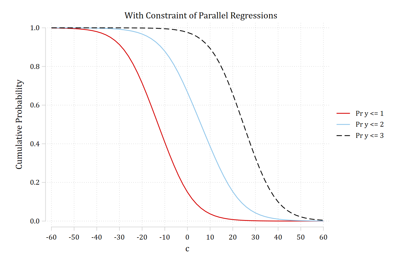
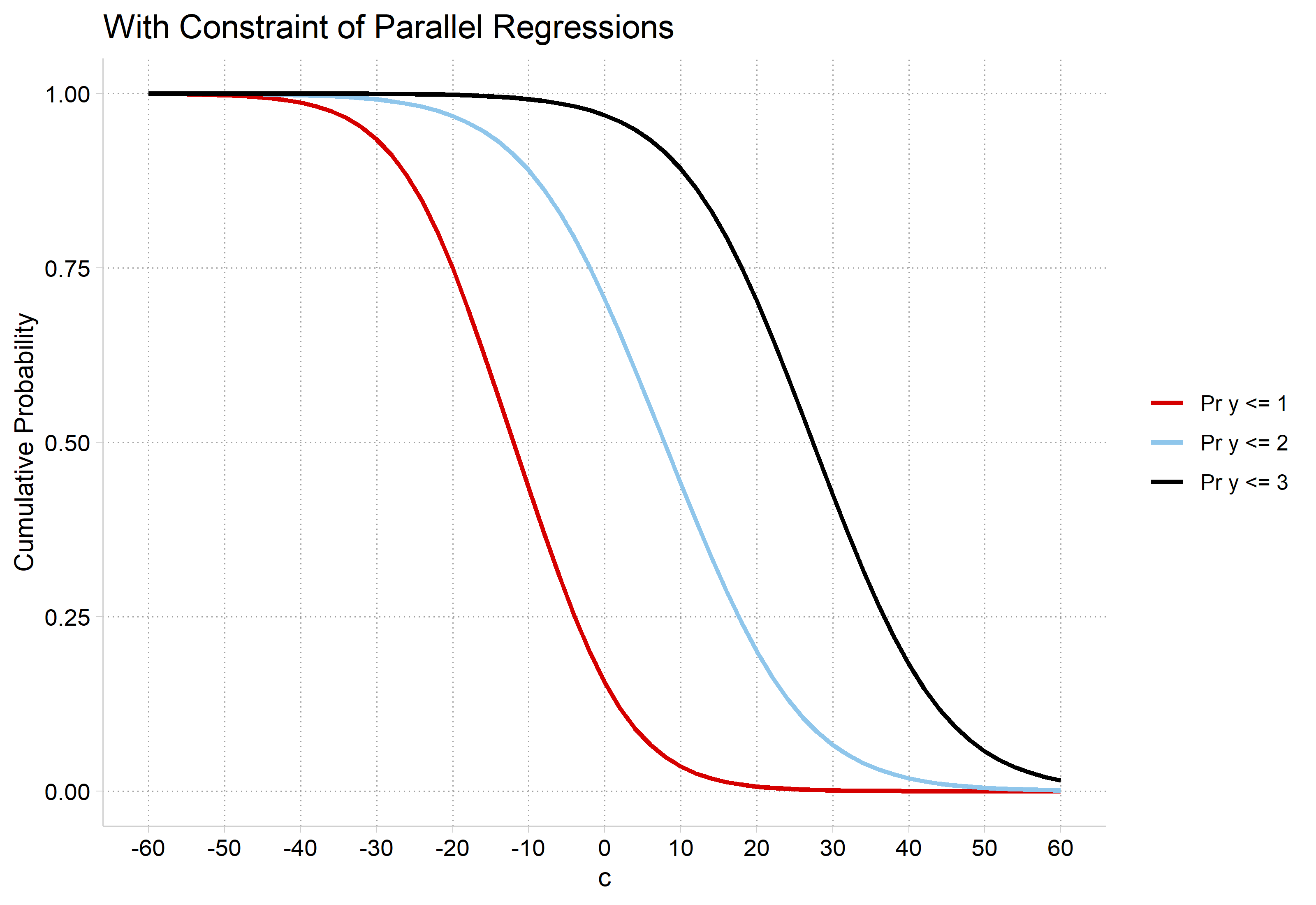
With the constraint of parallel regressions: three S-shaped cumulative probability curves for Pr(y ≤ 1), Pr(y ≤ 2), and Pr(y ≤ 3) fall from 1 to 0 across c with the same slope, shifted about 20 units apart.

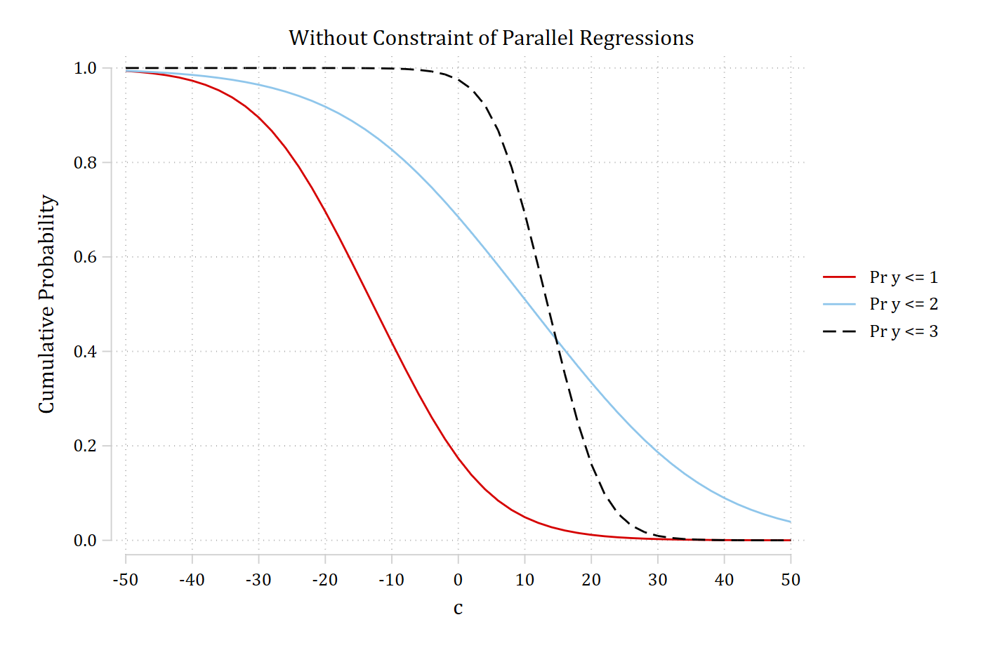
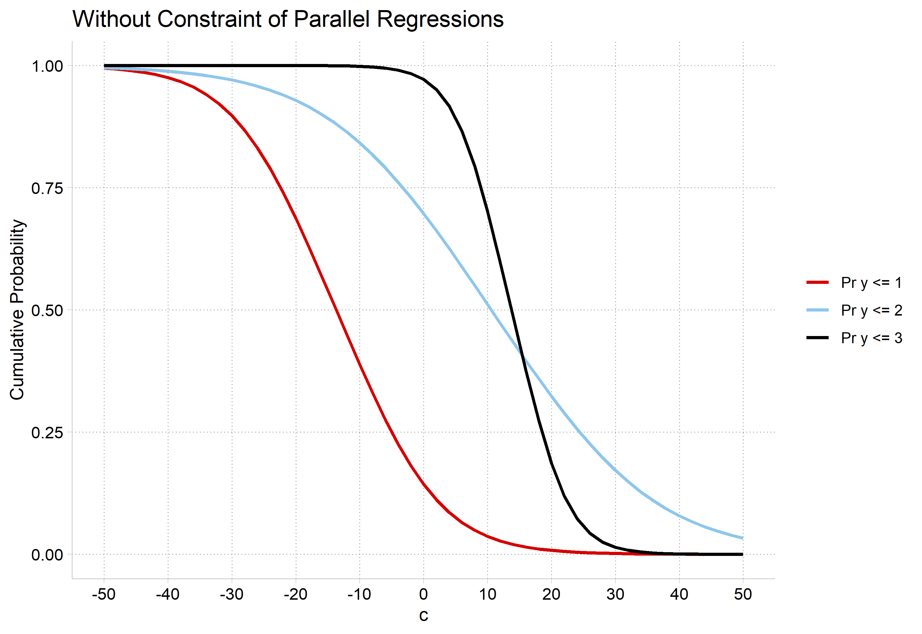
Without the constraint of parallel regressions: the three cumulative probability curves fall at different rates; Pr(y ≤ 2) is the flattest and Pr(y ≤ 3) the steepest, so the curves cross.

library(haven)           # import Stata data and labels
library(dplyr)           # data manipulation
library(sjmisc)          # frq() frequency tables
library(ggplot2)         # graphs
library(MASS)            # ordinal logit: polr(); mvrnorm()
library(nnet)            # multinomial logit: multinom()
library(marginaleffects) # predictions and marginal effects
library(brant)           # Brant test: brant()
library(car)             # Anova()
library(suest)           # combine models to compare MEs: suest()
library(cleanplots)      # graph scheme
cleanplots_defaults()

# Simulate data to show parallel regression assumption
# (R's random numbers differ from Stata's, so the estimates differ a little)
set.seed(30004)
n <- 2000
sim <- as.data.frame(mvrnorm(n, mu = c(0, 0), Sigma = matrix(c(1, .2, .2, 1), 2),
  empirical = TRUE))  # x1 and x2 with a small correlation
names(sim) <- c("x1", "x2")
sim <- sim |>
  mutate(c = rnorm(n, 0, 10),
    b = rep(0:1, each = n / 2),
    y1 = as.numeric(runif(n) < plogis(-3 - 0.15 * c + 2 * b)),
    y2 = as.numeric(runif(n) < plogis(0 - 0.15 * c + 2 * b)),
    y3 = as.numeric(runif(n) < plogis(3 - 0.15 * c + 2 * b)),
    y1A = as.numeric(runif(n) < plogis(-3 - 0.15 * c + 2 * b)),
    y2A = as.numeric(runif(n) < plogis(0 - 0.1 * c + 2 * b)),
    y3A = as.numeric(runif(n) < plogis(3 - 0.3 * c + 2 * b)))

# Average predicted Pr(y = 1) from a binary logit at values of c
cum_pr <- function(outcome, cvalues) {
  m <- glm(reformulate(c("c", "b", "x1", "x2"), outcome), data = sim, family = binomial)
  avg_predictions(m, by = "c", newdata = datagrid(c = cvalues, grid_type = "counterfactual"))
}
cum_labels <- c("Pr y <= 1", "Pr y <= 2", "Pr y <= 3")

# Parallel Regressions
parallel <- bind_rows(lapply(c("y1", "y2", "y3"), cum_pr, cvalues = seq(-60, 60, 2)),
  .id = "outcome")

ggplot(parallel, aes(x = c, y = estimate, color = outcome)) +
  geom_line(linewidth = 1) +
  scale_color_discrete(labels = cum_labels) +
  scale_x_continuous(breaks = seq(-60, 60, 10)) +
  labs(title = "With Constraint of Parallel Regressions",
    y = "Cumulative Probability", color = NULL)

With the constraint of parallel regressions: three S-shaped cumulative probability curves for Pr(y ≤ 1), Pr(y ≤ 2), and Pr(y ≤ 3) fall from 1 to 0 across c with the same slope, shifted about 20 units apart.

# w/o Parallel Regressions
nonparallel <- bind_rows(lapply(c("y1A", "y2A", "y3A"), cum_pr, cvalues = seq(-50, 50, 2)),
  .id = "outcome")

ggplot(nonparallel, aes(x = c, y = estimate, color = outcome)) +
  geom_line(linewidth = 1) +
  scale_color_discrete(labels = cum_labels) +
  scale_x_continuous(breaks = seq(-50, 50, 10)) +
  labs(title = "Without Constraint of Parallel Regressions",
    y = "Cumulative Probability", color = NULL)

Without the constraint of parallel regressions: the three cumulative probability curves fall at different rates; Pr(y ≤ 2) is the flattest and Pr(y ≤ 3) the steepest, so the curves cross.

Is the slope for Pr(y ≤ 2) significantly different from Pr(y ≤ 3)? Pr(y ≤ 1)? Etc.

Ordinality assumption revisited

  • To begin this section, I emphasized the ordinality assumption is about the relationship between the IVs and the DVs—it is an assumption about the model, not just about the DV
  • Even when your DV is clearly an inherently ordinal DV (e.g., educational degree attainment)—this does not mean your model will meet the ordinality assumption
  • Consider the graph above: this plots the cumulative probabilities across the range of a continuous IV
    • Some IVs may produce ordinal relationships with the DV
    • Some IVs may not
  • Thus, a DV itself can never satisfy the ordinality assumption of the model
    • E.g., A DV may pass the assumption in one model or sample, but not an alternative with different IVs, or in a different sample

Formal tests of parallel regressions

  • The Brant test determines if the coefficients from individual binary logits equal those from the ordinal logit model where they are all constrained to be equal
    • In Stata, spost13 command brant will calculate this for you; both for each individual IV and an overall test for the model; in R, package brant
  • Tests often reject the parallel regression assumption
    • In my experience, they are very sensitive to even minor deviations from perfectly parallel regressions
  • If rejected, verify the consequences of the assumption by comparing predictions from the ordinal model with a model that does not impose the parallel regression assumption (e.g., multinomial logit)
    • I would not publish results from ordinal logit when tests indicate a violation of the parallel regression assumption unless I can provide explicit evidence it does not bias conclusions

Brant test of the parallel regression assumption

use "https://tdmize.github.io/data/data/cda_gss", clear
(cda_gss.dta |  GSS 1972-2021 CDA - Categorical Data Analysis | date created 202
> 3)
lab def likertlab 1"StrAgree" 2"Agree" 3"Disagree" 4"StrDisag"
lab val pillok likertlab
gen religous = attend
(665 missing values generated)
lab var religous "Religious Attendee"
recode religous 0/3 = 0 4/8 = 1
(55,475 changes made to religous)
lab def religlab 0"Not Religious" 1"Religious"
lab val religous religlab
drop if year < 1986
(18,586 observations deleted)
drop if missing(pillok, year1972, religous, college, age, woman, race3, faminc
)
(25,267 observations deleted)
qui ologit pillok c.year1972 c.age i.woman i.religous ///
    i.college i.race3 c.faminc, or
est store opmod
// Test the parallel regression assumption
brant
Brant test of parallel regression assumption

              |       chi2     p>chi2      df
 -------------+------------------------------
          All |     100.80      0.000      16
 -------------+------------------------------
     year1972 |       0.77      0.681       2
          age |      23.89      0.000       2
      1.woman |      12.07      0.002       2
   1.religous |      37.95      0.000       2
    1.college |       8.64      0.013       2
      2.race3 |      12.00      0.002       2
      3.race3 |       1.42      0.492       2
       faminc |       1.01      0.605       2

A significant test statistic provides evidence that the parallel
regression assumption has been violated.
gss <- read_dta("https://tdmize.github.io/data/data/cda_gss.dta")

# Religious attendee = attends about once a month or more
gss <- gss |>
  mutate(religous = case_when(attend <= 3 ~ 0, attend >= 4 ~ 1)) |>
  filter(year >= 1986)

# Keep model variables; drop any missing data
gss <- gss[c("pillok", "year1972", "religous", "college", "age", "woman", "race3", "faminc")]
gss <- gss[complete.cases(gss), ]

# Ordinal DV as a factor with short labels; binary/nominal variables as factors
gss <- gss |>
  mutate(pillok = factor(pillok, levels = 1:4,
      labels = c("StrAgree", "Agree", "Disagree", "StrDisag")),
    religous = factor(religous, labels = c("Not Religious", "Religious")),
    across(c(college, woman, race3), as_factor),
    year1972 = as.numeric(year1972)) |>
  droplevels()

opmod <- polr(pillok ~ year1972 + age + woman + religous + college + race3 + faminc,
  data = gss, Hess = TRUE)

# Test the parallel regression assumption
brant(opmod)
---------------------------------------------------- 
Test for        X2  df  probability 
---------------------------------------------------- 
Omnibus         100.8   16  0
year1972        0.77    2   0.68
age         23.89   2   0
womanWomen      12.07   2   0
religousReligious   37.95   2   0
collegeCollege Degree   8.64    2   0.01
race3black      12.01   2   0
race3other      1.42    2   0.49
faminc          1.01    2   0.6
---------------------------------------------------- 

H0: Parallel Regression Assumption holds

A Brant test indicates that the model violates the parallel regression assumption of the ordinal logit model (p < 0.001). Age, gender, religiosity, education, and race all have relationships with views of teenage birth control that may not be strictly ordered in nature (all five individual tests p < 0.05).

Comparing ordinal and nominal predictions

  • Before blindly accepting or rejecting the ordinal logit model based on a test of parallel regressions, you should also examine whether predictions from the ordinal model differ importantly from those in a model that does not impose ordinality

Effects of assuming wrong level of measurement

Model choice (assumed level of DV for analysis) True level of DV: Nominal Ordinal Continuous*
Nominal Ideal Inefficient Inefficient
Ordinal Biased Ideal Inefficient
Continuous Biased Biased Ideal

*I am not distinguishing between interval and ratio variables here

  • If outcome is ordinal and model is nominal, it is inefficient, but a safe choice
    • If outcome is nominal but model is ordinal, you will have biased estimates
  • Here I compare ordinal logit to multinomial logit
    • You could also compare predictions to those from the generalized ordered logit model (see Section 5.6)
// Same model with mlogit //
qui mlogit pillok c.year1972 c.age i.woman i.religous ///
    i.college i.race3 c.faminc, rrr
est store mpmod
*5.4.a
qui margins, at(year1972=(14(1)49))
marginsplot, recastci(rline) ciopt(lpat(dash) col(*.5)) ///
    plotop(lwid(*1.5) msym(none)) ///
    ylab(0(.1).5) xtitle("GSS Survey Year") xlab(14 " " 18 28 38 49) ///
    ytitle("Pr(View of Birth Control for Teenagers)") ///
    title("[5.4.a] Multinomial Logit", size(large)) ///
    legend(order(5 "StrAgree" 6 "Agree" 7 "Disagree" 8 "StrDisag") ///
    rows(2) position(6)) saving(mlyear.gph, replace)
Variables that uniquely identify margins: year1972
(file mlyear.gph not found)
file mlyear.gph saved
*5.4.b
qui margins, at(age=(18(4)90))
marginsplot, recastci(rline) ciopt(lpat(dash) col(*.5)) ///
    plotop(lwid(*1.5) msym(none)) ylab(0(.1).5) ///
    xlabel(18(10)88, labsize(2.5)) xtitle("Age in Years") ///
    ytitle("Pr(View of Birth Control for Teenagers)") ///
    title("[5.4.b] Multinomial Logit", size(large)) ///
    legend(order(5 "StrAgree" 6 "Agree" 7 "Disagree" 8 "StrDisag") ///
    rows(2) position(6)) saving(mlage.gph, replace)
Variables that uniquely identify margins: age
(file mlage.gph not found)
file mlage.gph saved
*5.4.c
qui margins, dydx(woman)
marginsplot, recast(bar) ciopts(color(gs5)) ///
    xlab(0.5 " " 1 `" "Strongly" "Agree" "' 2 "Agree" ///
        3 "Disagree" 4 `" "Strongly" "Disagree" "' 4.5 " ") ///
    yline(0) plotopts(barw(0.6) color(ltblue)) ylab(-.1(.05).1, format(%4.2f))
 ///
    xtitle("Teenagers Should Have Birth Control?") ytitle("AME of Gender (Woma
n = 1)") ///
    title("[5.4.c] Multinomial Logit", size(large)) saving(mlwoman.gph, replac
e)
Variables that uniquely identify margins:
(file mlwoman.gph not found)
file mlwoman.gph saved
*5.4.d
qui margins, dydx(religous)
marginsplot, recast(bar) ciopts(color(gs5)) ///
    xlab(0.5 " " 1 `" "Strongly" "Agree" "' 2 "Agree" ///
        3 "Disagree" 4 `" "Strongly" "Disagree" "' 4.5 " ") ///
    yline(0) plotopts(barw(0.6) color(ltblue)) ylab(-.2(.05).2, format(%4.2f))
 ///
    xtitle("Teenagers Should Have Birth Control?") ytitle("AME of Religiosity 
(Religious = 1)") ///
    title("[5.4.d] Multinomial Logit", size(large)) saving(mlrelig.gph, replac
e)
Variables that uniquely identify margins:
(file mlrelig.gph not found)
file mlrelig.gph saved
*Same graphs from the ologit model
est restore opmod
(results opmod are active now)
*5.4.e
qui margins, at(year1972=(14(1)49))
marginsplot, recastci(rline) ciopt(lpat(dash) col(*.5)) ///
    plotop(lwid(*1.5) msym(none)) ///
    ylab(0(.1).5) xtitle("GSS Survey Year") xlab(14 " " 18 28 38 49) ///
    ytitle("Pr(View of Birth Control for Teenagers)") ///
    title("[5.4.e] Ordinal Logit", size(large)) ///
    legend(order(5 "StrAgree" 6 "Agree" 7 "Disagree" 8 "StrDisag") ///
    rows(2) position(6)) saving(olyear.gph, replace)
Variables that uniquely identify margins: year1972
(file olyear.gph not found)
file olyear.gph saved
*5.4.f
qui margins, at(age=(18(4)90))
marginsplot, recastci(rline) ciopt(lpat(dash) col(*.5)) ///
    plotop(lwid(*1.5) msym(none)) ylab(0(.1).5) ///
    xlabel(18(10)88, labsize(2.5)) xtitle("Age in Years") ///
    ytitle("Pr(View of Birth Control for Teenagers)") ///
    title("[5.4.f] Ordinal Logit", size(large)) ///
    legend(order(5 "StrAgree" 6 "Agree" 7 "Disagree" 8 "StrDisag") ///
    rows(2) position(6)) saving(olage.gph, replace)
Variables that uniquely identify margins: age
(file olage.gph not found)
file olage.gph saved
*5.4.g
qui margins, dydx(woman)
marginsplot, recast(bar) ciopts(color(gs5)) ///
    xlab(0.5 " " 1 `" "Strongly" "Agree" "' 2 "Agree" ///
        3 "Disagree" 4 `" "Strongly" "Disagree" "' 4.5 " ") ///
    yline(0) plotopts(barw(0.6) color(ltblue)) ylab(-.1(.05).1, format(%4.2f))
 ///
    xtitle("Teenagers Should Have Birth Control?") ytitle("AME of Gender (Woma
n = 1)") ///
    title("[5.4.g] Ordinal Logit", size(large)) saving(olwoman.gph, replace)
Variables that uniquely identify margins:
(file olwoman.gph not found)
file olwoman.gph saved
*5.4.h
qui margins, dydx(religous)
marginsplot, recast(bar) ciopts(color(gs5)) ///
    xlab(0.5 " " 1 `" "Strongly" "Agree" "' 2 "Agree" ///
        3 "Disagree" 4 `" "Strongly" "Disagree" "' 4.5 " ") ///
    yline(0) plotopts(barw(0.6) color(ltblue)) ylab(-.2(.05).2, format(%4.2f))
 ///
    xtitle("Teenagers Should Have Birth Control?") ytitle("AME of Religiosity 
(Religious = 1)") ///
    title("[5.4.h] Ordinal Logit", size(large)) saving(olrelig.gph, replace)
Variables that uniquely identify margins:
(file olrelig.gph not found)
file olrelig.gph saved
** Combine ologit and mlogit graphs to compare **
graph combine olyear.gph mlyear.gph
graph combine olage.gph mlage.gph
graph combine olwoman.gph mlwoman.gph
graph combine olrelig.gph mlrelig.gph

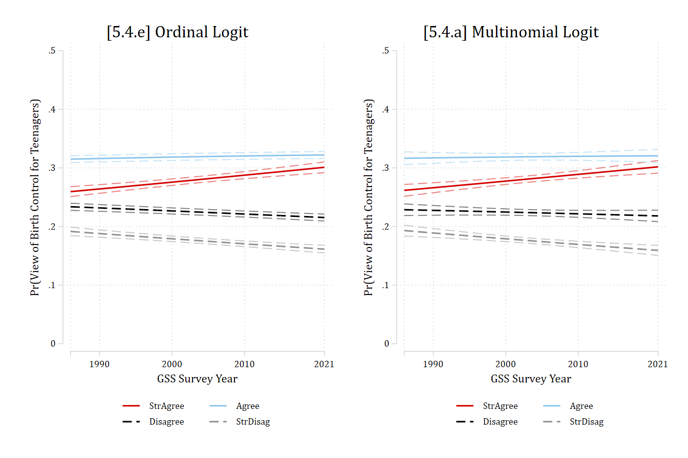
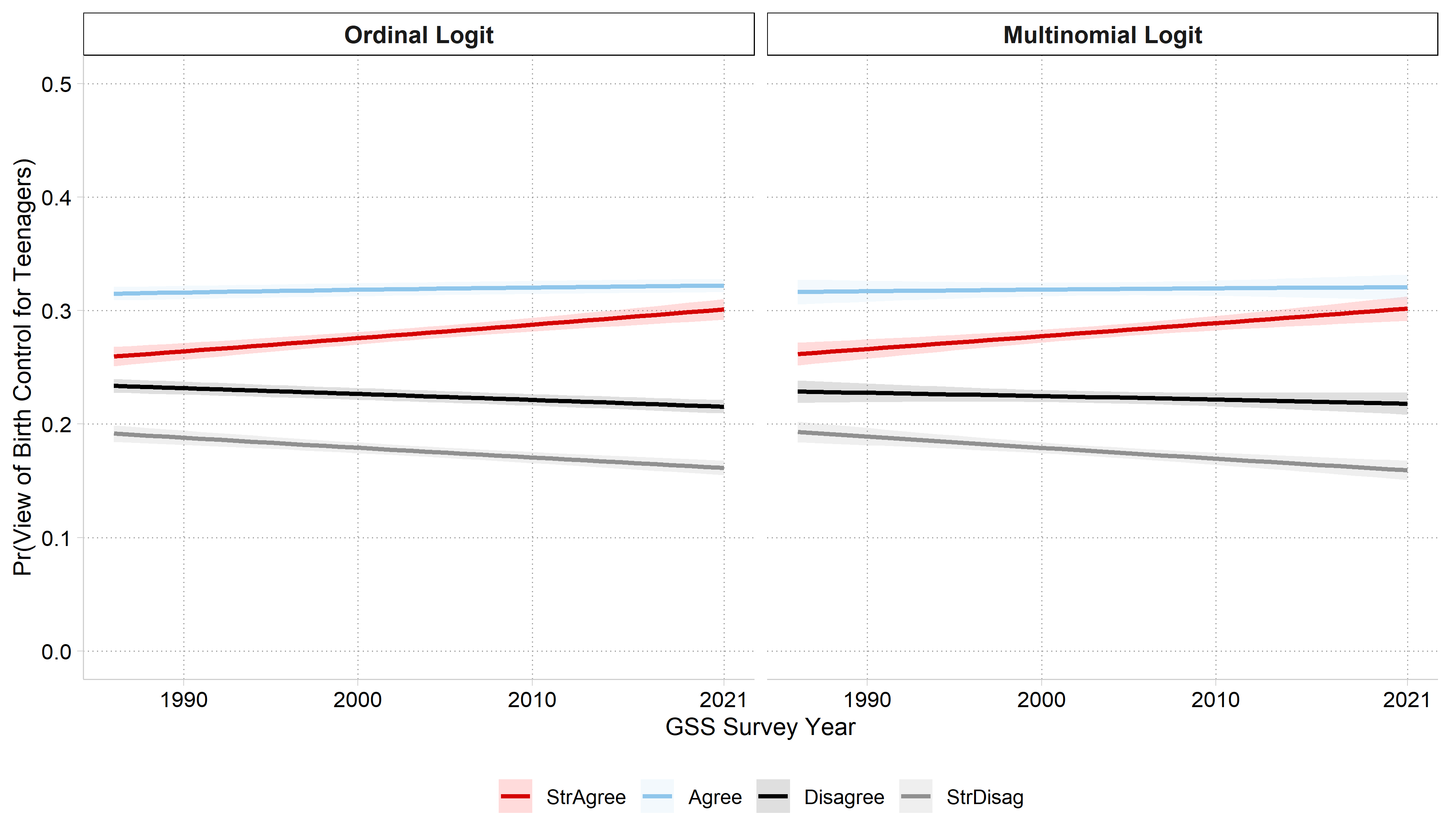
[5.4.e] ordinal logit and [5.4.a] multinomial logit predicted probabilities of each view by survey year side by side: the two models give nearly the same, nearly flat lines.

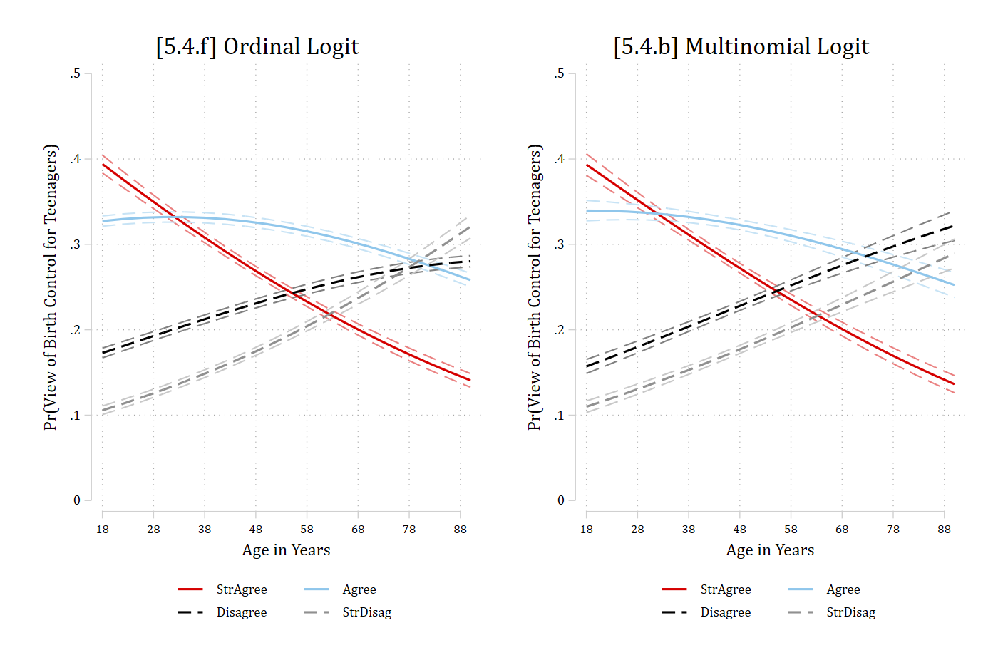
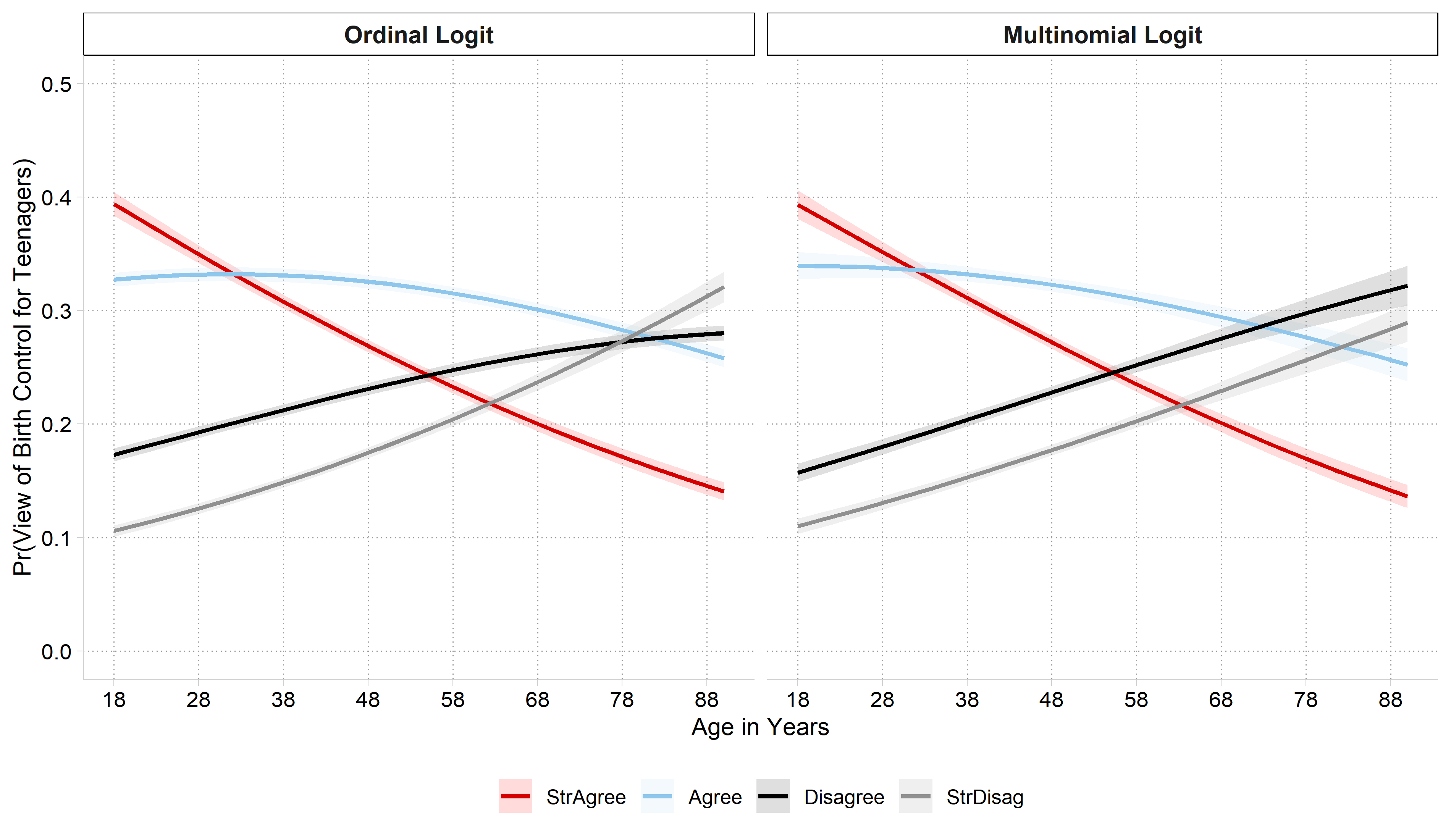
[5.4.f] ordinal logit and [5.4.b] multinomial logit predicted probabilities of each view by age side by side: both show strongly agree falling and strongly disagree rising with age; the multinomial model has disagree rising faster and strongly disagree rising slower than the ordinal model.

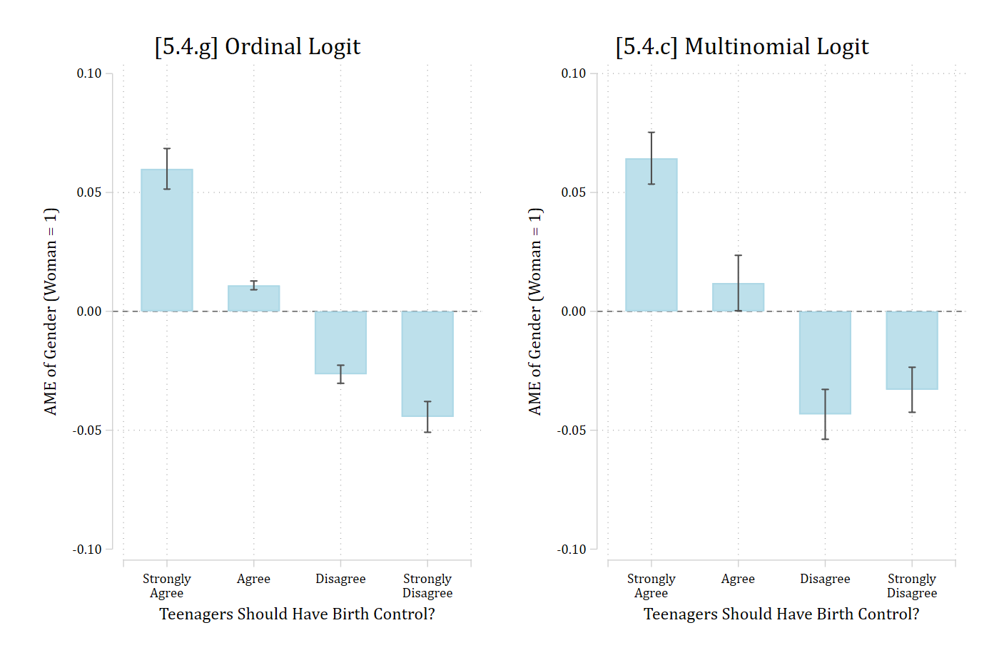
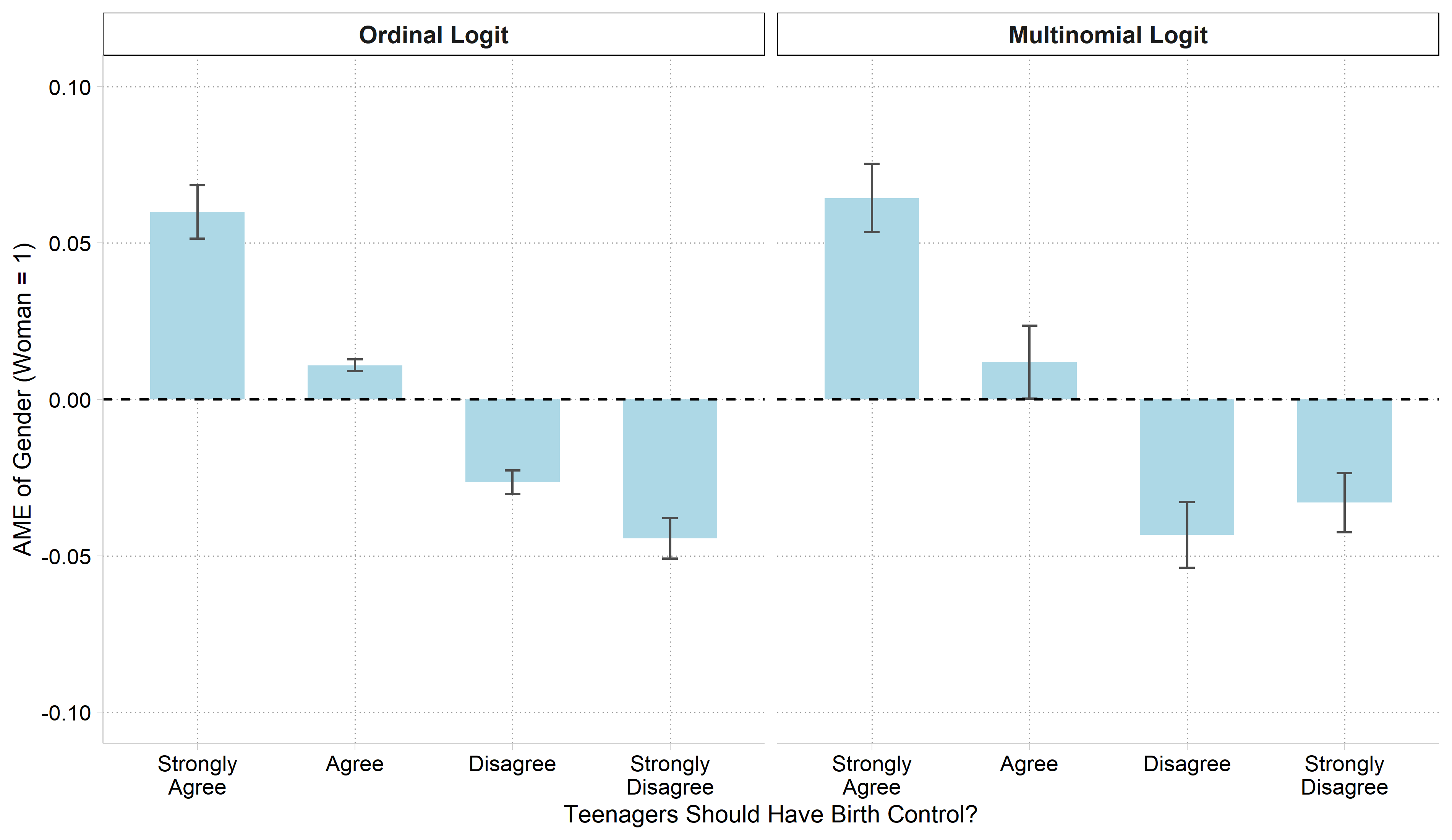
[5.4.g] ordinal logit and [5.4.c] multinomial logit average marginal effects of gender on each view side by side: both have positive effects for strongly agree and agree and negative effects for disagree and strongly disagree, but the multinomial model's effect for disagree is larger and for strongly disagree smaller.

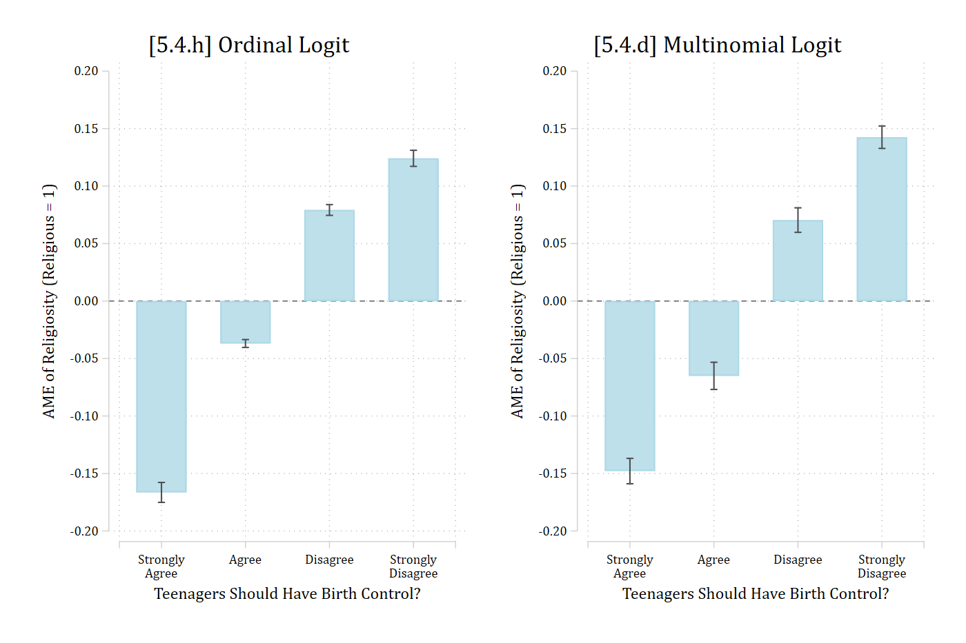
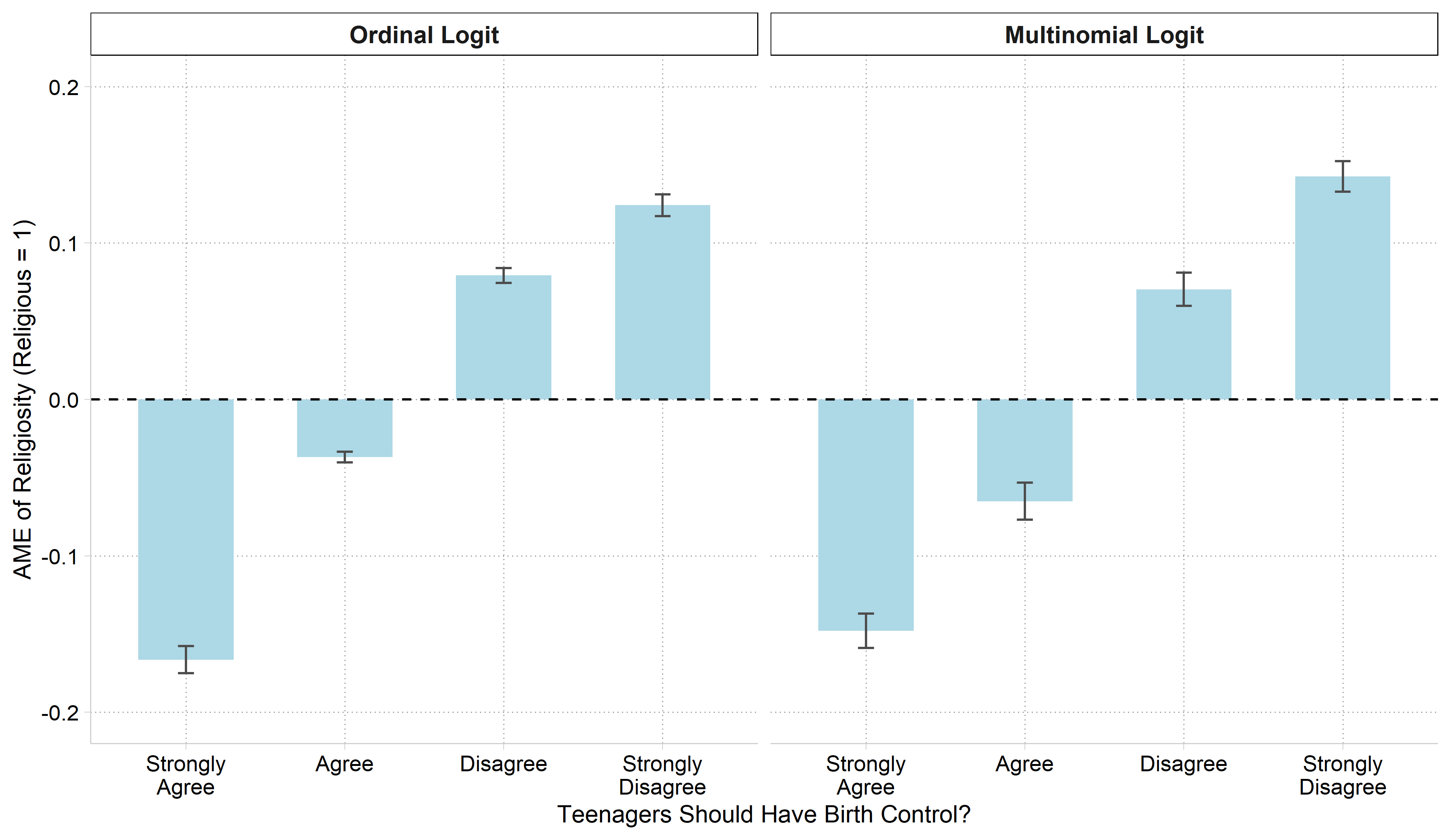
[5.4.h] ordinal logit and [5.4.d] multinomial logit average marginal effects of religiosity on each view side by side: both are negative for strongly agree and agree and positive for disagree and strongly disagree; the multinomial model has a larger negative effect for agree and a larger positive effect for strongly disagree.

# Same model with multinomial logit
mpmod <- multinom(pillok ~ year1972 + age + woman + religous + college + race3 + faminc,
  data = gss, trace = FALSE)

# Average predictions from both models at values of an IV
pr_both <- function(variable, values) {
  grid <- do.call(datagrid, c(list(newdata = gss, grid_type = "counterfactual"),
    setNames(list(values), variable)))
  bind_rows(
    "Ordinal Logit" = avg_predictions(opmod, by = c(variable, "group"), newdata = grid),
    "Multinomial Logit" = avg_predictions(mpmod, by = c(variable, "group"), newdata = grid),
    .id = "model") |>
    mutate(model = factor(model, levels = c("Ordinal Logit", "Multinomial Logit")))
}

# 5.4.e and 5.4.a
ggplot(pr_both("year1972", 14:49), aes(x = year1972, y = estimate, color = group)) +
  geom_ribbon(aes(ymin = conf.low, ymax = conf.high, fill = group), alpha = .2, color = NA) +
  geom_line(linewidth = 1) +
  facet_wrap(~ model) +
  scale_x_continuous(breaks = c(18, 28, 38, 49), labels = c("1990", "2000", "2010", "2021")) +
  scale_y_continuous(breaks = seq(0, .5, .1), limits = c(0, .5)) +
  labs(x = "GSS Survey Year", y = "Pr(View of Birth Control for Teenagers)",
    color = NULL, fill = NULL) +
  theme(legend.position = "bottom")

[5.4.e] ordinal logit and [5.4.a] multinomial logit predicted probabilities of each view by survey year side by side: the two models give nearly the same, nearly flat lines.

# 5.4.f and 5.4.b
ggplot(pr_both("age", seq(18, 90, 4)), aes(x = age, y = estimate, color = group)) +
  geom_ribbon(aes(ymin = conf.low, ymax = conf.high, fill = group), alpha = .2, color = NA) +
  geom_line(linewidth = 1) +
  facet_wrap(~ model) +
  scale_x_continuous(breaks = seq(18, 88, 10)) +
  scale_y_continuous(breaks = seq(0, .5, .1), limits = c(0, .5)) +
  labs(x = "Age in Years", y = "Pr(View of Birth Control for Teenagers)",
    color = NULL, fill = NULL) +
  theme(legend.position = "bottom")

[5.4.f] ordinal logit and [5.4.b] multinomial logit predicted probabilities of each view by age side by side: both show strongly agree falling and strongly disagree rising with age; the multinomial model has disagree rising faster and strongly disagree rising slower than the ordinal model.

# AMEs from both models
me_both <- function(variable) {
  bind_rows(
    "Ordinal Logit" = avg_comparisons(opmod, variables = variable),
    "Multinomial Logit" = avg_comparisons(mpmod, variables = variable),
    .id = "model") |>
    mutate(model = factor(model, levels = c("Ordinal Logit", "Multinomial Logit")))
}

ame_plot <- function(mes, ytitle, ylimits) {
  ggplot(mes, aes(x = group, y = estimate)) +
    geom_col(width = .6, fill = "lightblue") +
    geom_errorbar(aes(ymin = conf.low, ymax = conf.high), width = .1, color = "gray30") +
    geom_hline(yintercept = 0, linetype = "dashed") +
    facet_wrap(~ model) +
    scale_x_discrete(labels = c("Strongly\nAgree", "Agree", "Disagree", "Strongly\nDisagree")) +
    scale_y_continuous(limits = ylimits) +
    labs(x = "Teenagers Should Have Birth Control?", y = ytitle)
}

# 5.4.g and 5.4.c
ame_plot(me_both("woman"), "AME of Gender (Woman = 1)", c(-.1, .1))

[5.4.g] ordinal logit and [5.4.c] multinomial logit average marginal effects of gender on each view side by side: both have positive effects for strongly agree and agree and negative effects for disagree and strongly disagree, but the multinomial model's effect for disagree is larger and for strongly disagree smaller.

# 5.4.h and 5.4.d
ame_plot(me_both("religous"), "AME of Religiosity (Religious = 1)", c(-.2, .2))

[5.4.h] ordinal logit and [5.4.d] multinomial logit average marginal effects of religiosity on each view side by side: both are negative for strongly agree and agree and positive for disagree and strongly disagree; the multinomial model has a larger negative effect for agree and a larger positive effect for strongly disagree.

Comparing model predicted probabilities

  • The plots above compare AMEs and ranges of predictions for particular independent variables.
  • It can also be informative to examine predicted probabilities for individual observations
    • E.g., What is the Pr(Agree) for observation #103 when using ologit vs mlogit?
// 5.4.i - Compare predictions for individual obs
est restore mpmod
(results mpmod are active now)
predict mpr1 mpr2 mpr3 mpr4
(option pr assumed; predicted probabilities)
est restore opmod
(results opmod are active now)
predict opr1 opr2 opr3 opr4
(option pr assumed; predicted probabilities)
scatter mpr1 opr1, jitter(2) xlab(0(.1).6) ylab(0(.1).6) msize(vsmall) ///
    xtitle("Pr(StrAgree) from Ordinal Logit") ytitle("Pr(StrAgree) Multinomial
 Logit") ///
    saving(pr1.gph, replace)
(file pr1.gph not found)
file pr1.gph saved
scatter mpr2 opr2, jitter(2) xlab(0(.1).6) ylab(0(.1).6) msize(vsmall) ///
    xtitle("Pr(Agree) from Ordinal Logit") ytitle("Pr(Agree) Multinomial Logit
") ///
    saving(pr2.gph, replace)
(file pr2.gph not found)
file pr2.gph saved
scatter mpr3 opr3, jitter(2) xlab(0(.1).6) ylab(0(.1).6) msize(vsmall) ///
    xtitle("Pr(Disagree) from Ordinal Logit") ytitle("Pr(Disagree) Multinomial
 Logit") ///
    saving(pr3.gph, replace)
(file pr3.gph not found)
file pr3.gph saved
scatter mpr4 opr4, jitter(2) xlab(0(.1).6) ylab(0(.1).6) msize(vsmall) ///
    xtitle("Pr(StrDisagree) from Ordinal Logit") ytitle("Pr(StrDisagree) Multi
nomial Logit") ///
    saving(pr4.gph, replace)
(file pr4.gph not found)
file pr4.gph saved
graph combine pr1.gph pr2.gph pr3.gph pr4.gph, ///
    title("[5.4.i] Predicted Probabilities from Multinomial Logit (y-axis)" //
/
        "vs Ordinal Logit (x-axis)", size(medsmall))

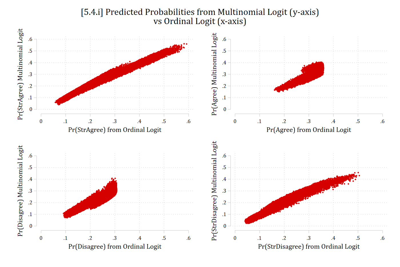
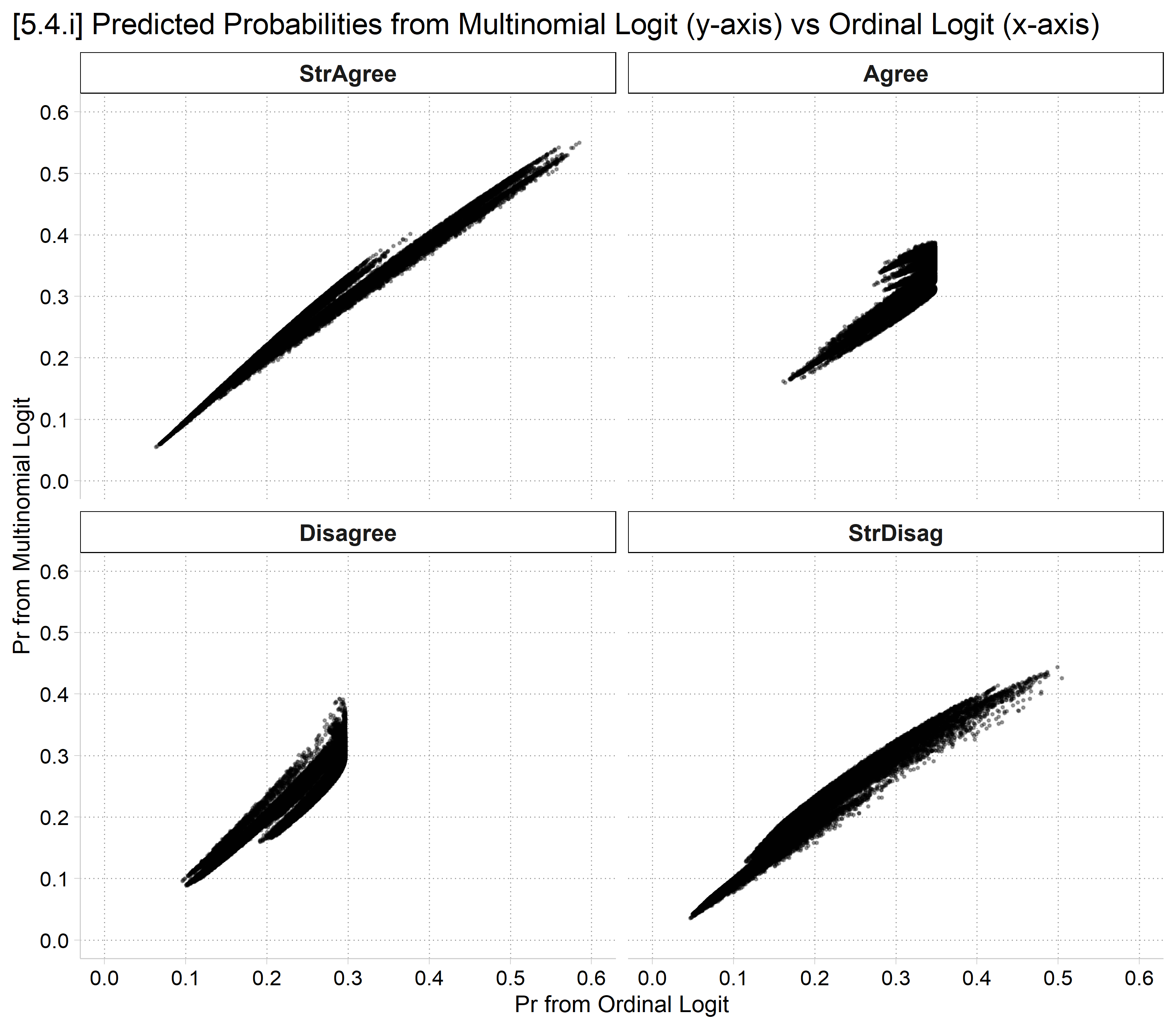
[5.4.i] Four scatterplots of each observation's predicted probability from the multinomial logit (y-axis) against the ordinal logit (x-axis): strongly agree and strongly disagree fall close to a straight line, while agree and disagree spread out more, especially at the higher ordinal-logit predictions.

# 5.4.i - Compare predictions for individual obs
pr_obs <- data.frame(outcome = rep(levels(gss$pillok), each = nrow(gss)),
  multinomial = as.vector(predict(mpmod, type = "probs")),
  ordinal = as.vector(predict(opmod, type = "probs"))) |>
  mutate(outcome = factor(outcome, levels = levels(gss$pillok)))

ggplot(pr_obs, aes(x = ordinal, y = multinomial)) +
  geom_point(size = .3, alpha = .3) +
  facet_wrap(~ outcome) +
  scale_x_continuous(breaks = seq(0, .6, .1), limits = c(0, .6)) +
  scale_y_continuous(breaks = seq(0, .6, .1), limits = c(0, .6)) +
  labs(title = "[5.4.i] Predicted Probabilities from Multinomial Logit (y-axis) vs Ordinal Logit (x-axis)",
    x = "Pr from Ordinal Logit", y = "Pr from Multinomial Logit") +
  theme(plot.title.position = "plot")

[5.4.i] Four scatterplots of each observation's predicted probability from the multinomial logit (y-axis) against the ordinal logit (x-axis): strongly agree and strongly disagree fall close to a straight line, while agree and disagree spread out more, especially at the higher ordinal-logit predictions.

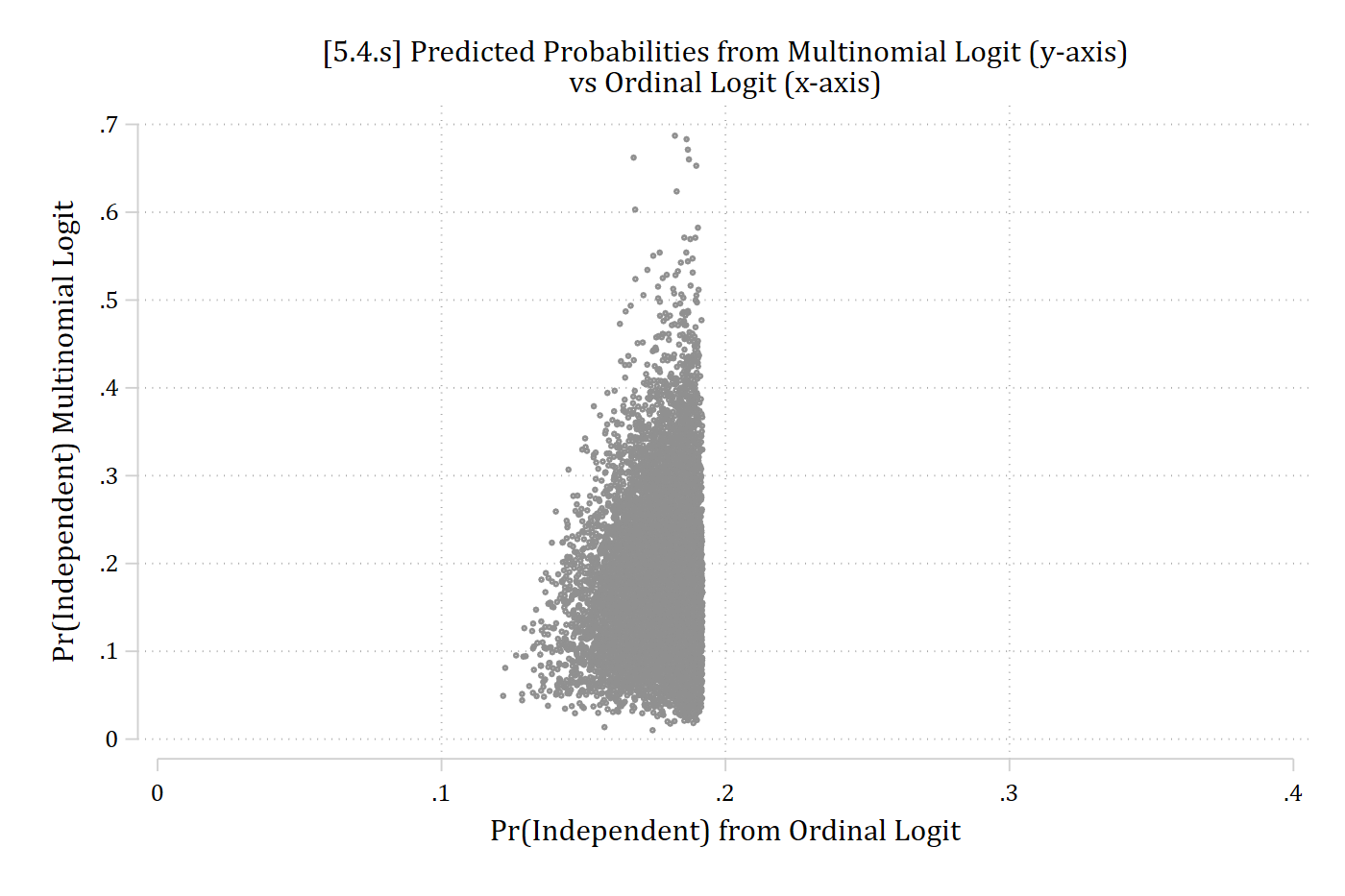
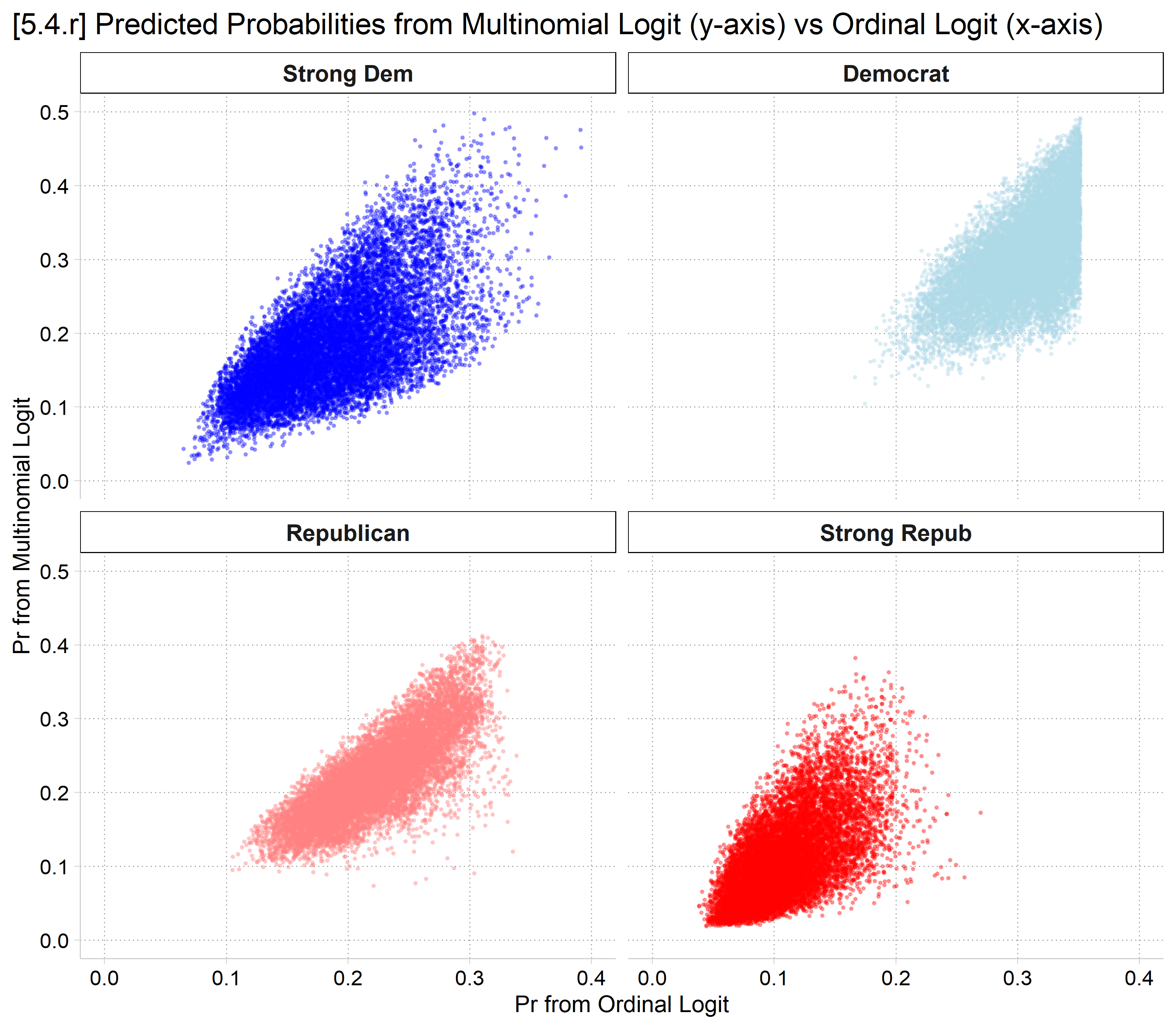
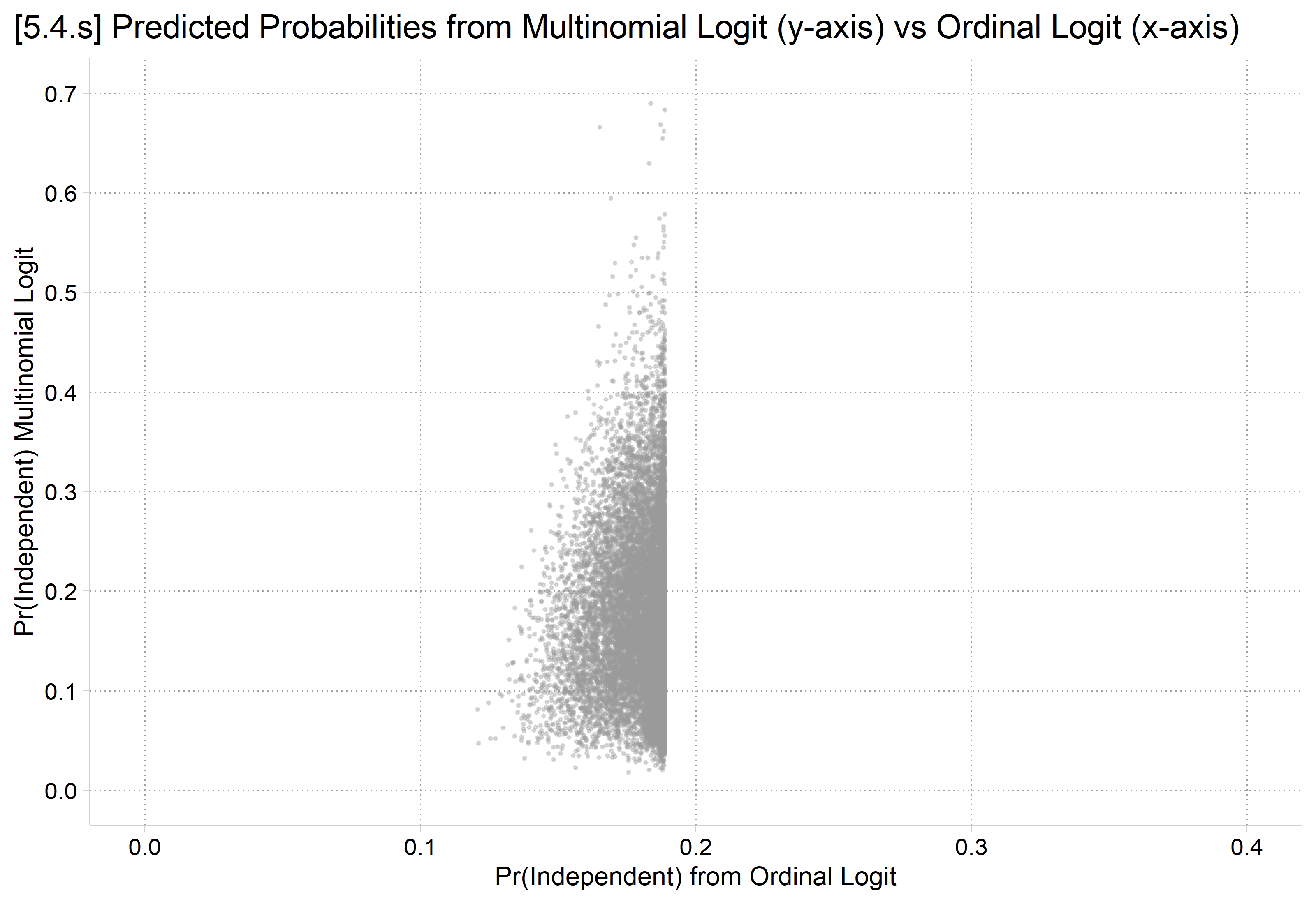
Where do the ordinal and multinomial models differ the most? Why?

Example: Political party affiliation*

  • GSS 2010 – 2021
    • DV: Political party affiliation
    • IVs: Age and gender
    • Control variables: education, parental status, marital status, family income, employment status, US region, and survey year
*2010 - 2021 GSS
use "https://tdmize.github.io/data/data/cda_gss", clear
(cda_gss.dta |  GSS 1972-2021 CDA - Categorical Data Analysis | date created 202
> 3)
drop if year < 2010
(53,043 observations deleted)
drop if missing(partyid5, woman, edyrs, age, parent, married, ///
    faminc, employed, region4, year)
(2,373 observations deleted)
fre partyid5
partyid5 -- Political Party Affiliation
--------------------------------------------------------------------
                       |      Freq.    Percent      Valid       Cum.
-----------------------+--------------------------------------------
Valid   0 Strong Dem   |       2504      18.64      18.64      18.64
        1 Democrat     |       4081      30.39      30.39      49.03
        2 Independent  |       2400      17.87      17.87      66.90
        3 Republican   |       2993      22.29      22.29      89.19
        4 Strong Repub |       1452      10.81      10.81     100.00
        Total          |      13430     100.00     100.00           
--------------------------------------------------------------------
party <- read_dta("https://tdmize.github.io/data/data/cda_gss.dta")
party <- party |> filter(year >= 2010)

# Keep model variables; drop any missing data
party <- party[c("partyid5", "woman", "edyrs", "age", "parent", "married", "faminc",
  "employed", "region4", "year")]
party <- party[complete.cases(party), ]

frq(party$partyid5)
Political Party Affiliation (x) <numeric> 
# total N=13430 valid N=13430 mean=1.76 sd=1.28

Value |        Label |    N | Raw % | Valid % | Cum. %
------------------------------------------------------
    0 |   Strong Dem | 2504 | 18.64 |   18.64 |  18.64
    1 |     Democrat | 4081 | 30.39 |   30.39 |  49.03
    2 |  Independent | 2400 | 17.87 |   17.87 |  66.90
    3 |   Republican | 2993 | 22.29 |   22.29 |  89.19
    4 | Strong Repub | 1452 | 10.81 |   10.81 | 100.00
 <NA> |         <NA> |    0 |  0.00 |    <NA> |   <NA>
# Outcome as a factor (and an ordered factor for polr); IVs as factors
party <- party |>
  mutate(partyid5 = as_factor(partyid5),
    party_ord = ordered(partyid5),
    across(c(woman, parent, married, employed, region4), as_factor),
    year = factor(year)) |>
  droplevels() |>
  as.data.frame()

*This example is an updated example of that shown in Long and Freese 2014 who use data from the 1992 National Election Study; this specific example from Mize, Doan, and Long 2019

Ordinal logit: DV = political party affiliation

///////////////////
// Ordinal Logit //
///////////////////
ologit partyid5 c.age i.woman c.edyrs i.parent i.married ///
    c.faminc i.employed i.region4 i.year, or
Iteration 0:  Log likelihood = -20922.836  
Iteration 1:  Log likelihood = -20679.067  
Iteration 2:  Log likelihood = -20678.564  
Iteration 3:  Log likelihood = -20678.564  

Ordered logistic regression                             Number of obs = 13,430
                                                        LR chi2(15)   = 488.54
                                                        Prob > chi2   = 0.0000
Log likelihood = -20678.564                             Pseudo R2     = 0.0117

------------------------------------------------------------------------------
    partyid5 | Odds ratio   Std. err.      z    P>|z|     [95% conf. interval]
-------------+----------------------------------------------------------------
         age |      1.000      0.001    0.190   0.849        0.998       1.002
             |
       woman |
      Women  |      0.766      0.024   -8.418   0.000        0.720       0.815
       edyrs |      0.953      0.005   -8.447   0.000        0.942       0.963
             |
      parent |
     Parent  |      1.126      0.043    3.081   0.002        1.044       1.215
             |
     married |
    Married  |      1.458      0.051   10.867   0.000        1.362       1.561
      faminc |      1.003      0.001    5.962   0.000        1.002       1.004
             |
    employed |
        Yes  |      1.084      0.037    2.360   0.018        1.014       1.160
             |
     region4 |
    Midwest  |      1.313      0.066    5.449   0.000        1.191       1.449
      South  |      1.384      0.064    7.009   0.000        1.263       1.515
       West  |      1.152      0.058    2.832   0.005        1.045       1.271
             |
        year |
       2012  |      0.938      0.057   -1.060   0.289        0.833       1.056
       2014  |      1.023      0.058    0.409   0.682        0.916       1.143
       2016  |      1.035      0.057    0.631   0.528        0.929       1.154
       2018  |      1.099      0.064    1.637   0.102        0.981       1.231
       2021  |      0.984      0.053   -0.308   0.758        0.885       1.093
-------------+----------------------------------------------------------------
       /cut1 |     -1.685      0.110                        -1.900      -1.469
       /cut2 |     -0.217      0.108                        -0.429      -0.005
       /cut3 |      0.547      0.108                         0.334       0.760
       /cut4 |      1.982      0.111                         1.765       2.200
------------------------------------------------------------------------------
Note: Estimates are transformed only in the first equation to odds ratios.
est store oparty
# Ordinal Logit
oparty <- polr(party_ord ~ age + woman + edyrs + parent + married + faminc + employed +
  region4 + year, data = party, Hess = TRUE)
summary(oparty)
Call:
polr(formula = party_ord ~ age + woman + edyrs + parent + married + 
    faminc + employed + region4 + year, data = party, Hess = TRUE)

Coefficients:
                    Value Std. Error t value
age             0.0001942  0.0010223  0.1899
womanWomen     -0.2666211  0.0316713 -8.4184
edyrs          -0.0486148  0.0057552 -8.4471
parentParent    0.1189137  0.0385979  3.0808
marriedMarried  0.3771437  0.0347073 10.8664
faminc          0.0031032  0.0005207  5.9596
employedYes     0.0810653  0.0343514  2.3599
region4Midwest  0.2725194  0.0500124  5.4490
region4South    0.3246471  0.0463160  7.0094
region4West     0.1416117  0.0500108  2.8316
year2012       -0.0640763  0.0604676 -1.0597
year2014        0.0231194  0.0564797  0.4093
year2016        0.0348560  0.0552461  0.6309
year2018        0.0946500  0.0578279  1.6368
year2021       -0.0165873  0.0539121 -0.3077

Intercepts:
                        Value    Std. Error t value 
Strong Dem|Democrat      -1.6846   0.1099   -15.3228
Democrat|Independent     -0.2168   0.1082    -2.0034
Independent|Republican    0.5470   0.1084     5.0437
Republican|Strong Repub   1.9822   0.1111    17.8479

Residual Deviance: 41357.13 
AIC: 41395.13 
# Odds ratios
exp(coef(oparty))
           age     womanWomen          edyrs   parentParent marriedMarried         faminc 
     1.0001942      0.7659632      0.9525480      1.1262727      1.4581138      1.0031080 
   employedYes region4Midwest   region4South    region4West       year2012       year2014 
     1.0844417      1.3132689      1.3835424      1.1521292      0.9379334      1.0233887 
      year2016       year2018       year2021 
     1.0354706      1.0992740      0.9835495 
  • In terms of the coefficients (y*):
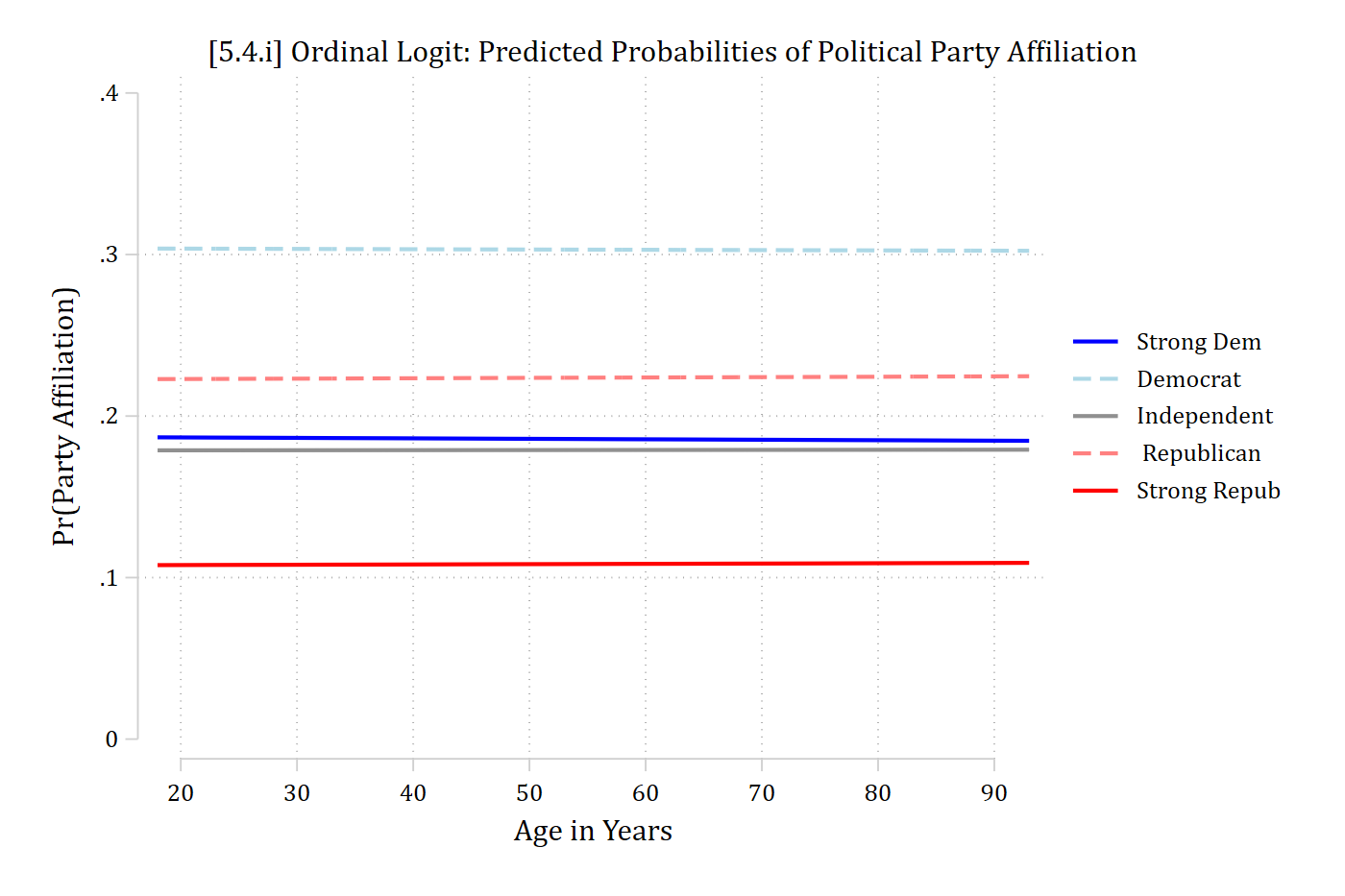
    • Age has no effect on the odds of political party affiliation
    • Women are less likely to identify as more Republican

AMEs from ordinal logit model

mchange age woman, amount(sd)
ologit: Changes in Pr(y) | Number of obs = 13430

Expression: Pr(partyid5), predict(outcome())

              | Strong ~m   Democrat  Indepen~t  Republi~n  Strong ~b 
--------------+------------------------------------------------------
age           |                                                      
          +SD |    -0.000     -0.000      0.000      0.000      0.000 
      p-value |     0.849      0.850      0.849      0.849      0.850 
woman         |                                                      
 Women vs Men |     0.039      0.026     -0.007     -0.032     -0.026 
      p-value |     0.000      0.000      0.000      0.000      0.000 

Average predictions

             | Strong ~m   Democrat  Indepen~t  Republi~n  Strong ~b 
-------------+------------------------------------------------------
  Pr(y|base) |     0.186      0.303      0.179      0.224      0.108 
# AMEs (mchange's +SD change starts at each observation's value)
avg_comparisons(oparty, variables = list(age = sd(party$age)))

        Group  Estimate Std. Error      z Pr(>|z|)   S     2.5 %  97.5 %
 Strong Dem   -4.99e-04   0.002625 -0.190    0.849 0.2 -0.005643 0.00465
 Democrat     -3.16e-04   0.001669 -0.190    0.850 0.2 -0.003587 0.00295
 Independent   8.93e-05   0.000468  0.191    0.849 0.2 -0.000828 0.00101
 Republican    4.05e-04   0.002133  0.190    0.849 0.2 -0.003776 0.00459
 Strong Repub  3.21e-04   0.001692  0.190    0.850 0.2 -0.002996 0.00364

Term: age
Type: probs
Comparison: +17.2933969697999
avg_comparisons(oparty, variables = "woman")

        Group Estimate Std. Error     z Pr(>|z|)    S    2.5 %   97.5 %
 Strong Dem    0.03930   0.004641  8.47   <0.001 55.1  0.03020  0.04839
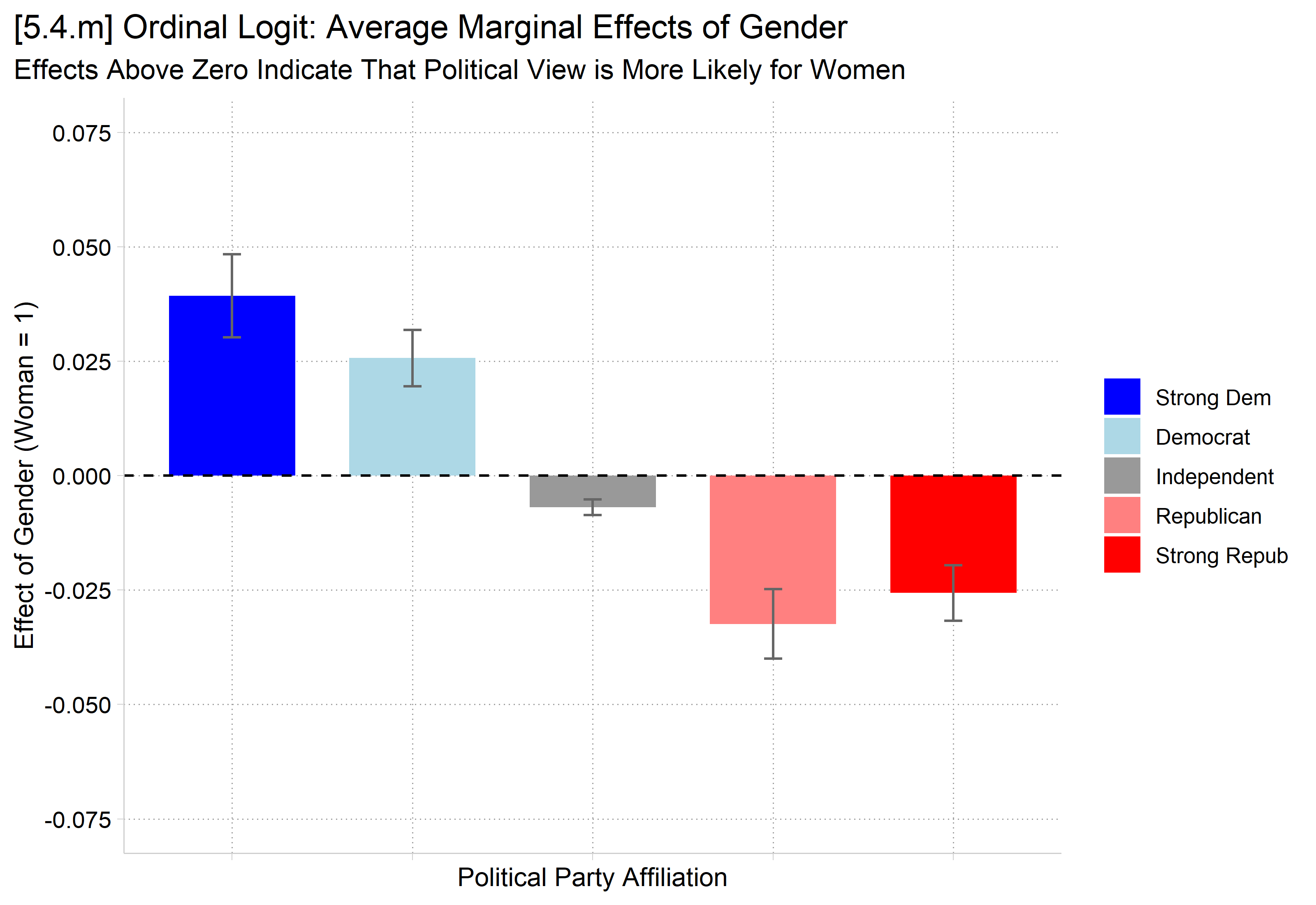
 Democrat      0.02569   0.003140  8.18   <0.001 51.7  0.01954  0.03185
 Independent  -0.00693   0.000875 -7.93   <0.001 48.6 -0.00865 -0.00522
 Republican   -0.03241   0.003881 -8.35   <0.001 53.7 -0.04002 -0.02480
 Strong Repub -0.02564   0.003108 -8.25   <0.001 52.5 -0.03174 -0.01955

Term: woman
Type: probs
Comparison: Women - Men
  • In terms of AMEs:
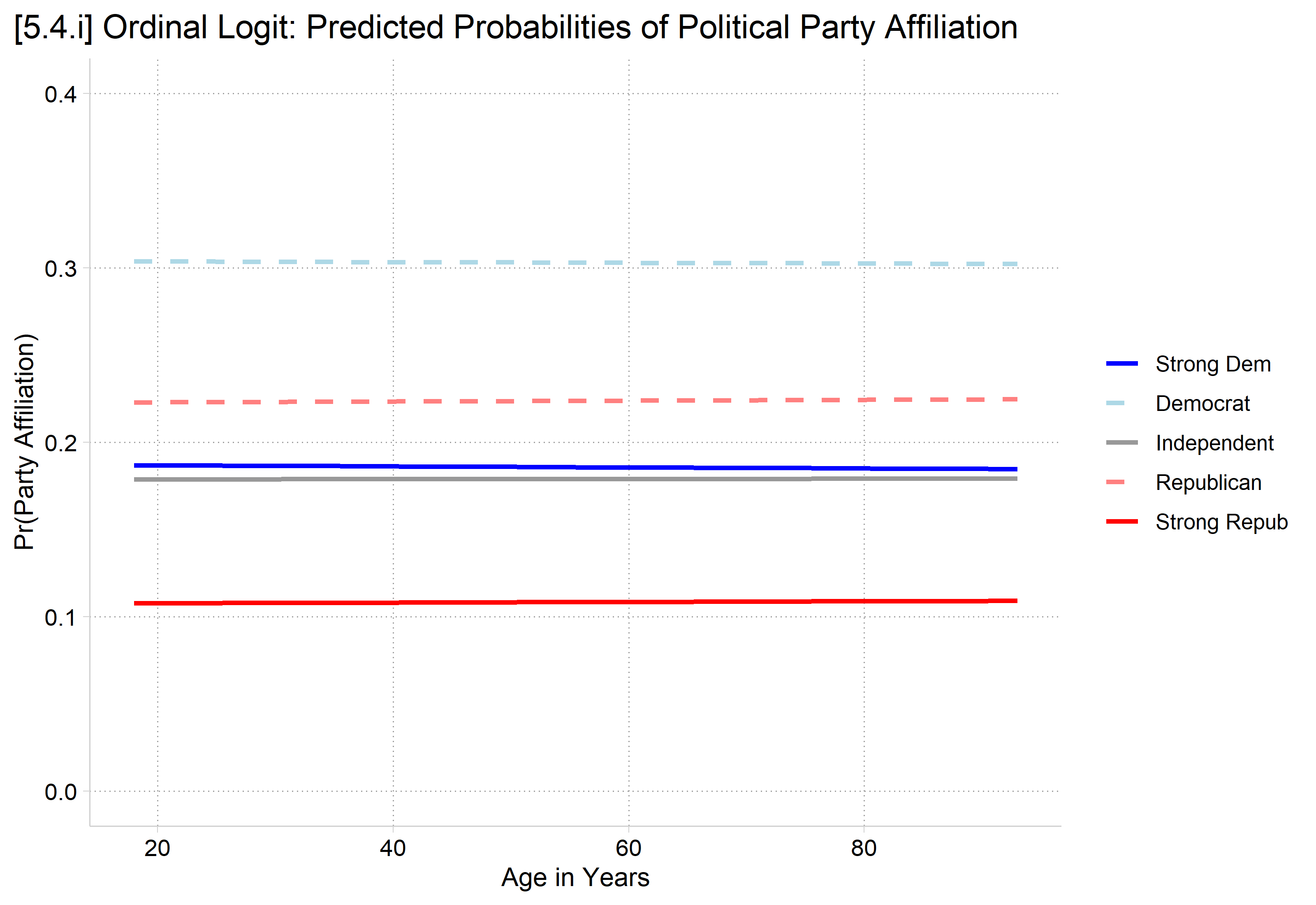
    • Age has no effect on the probability of identifying with any of the five political party affiliations
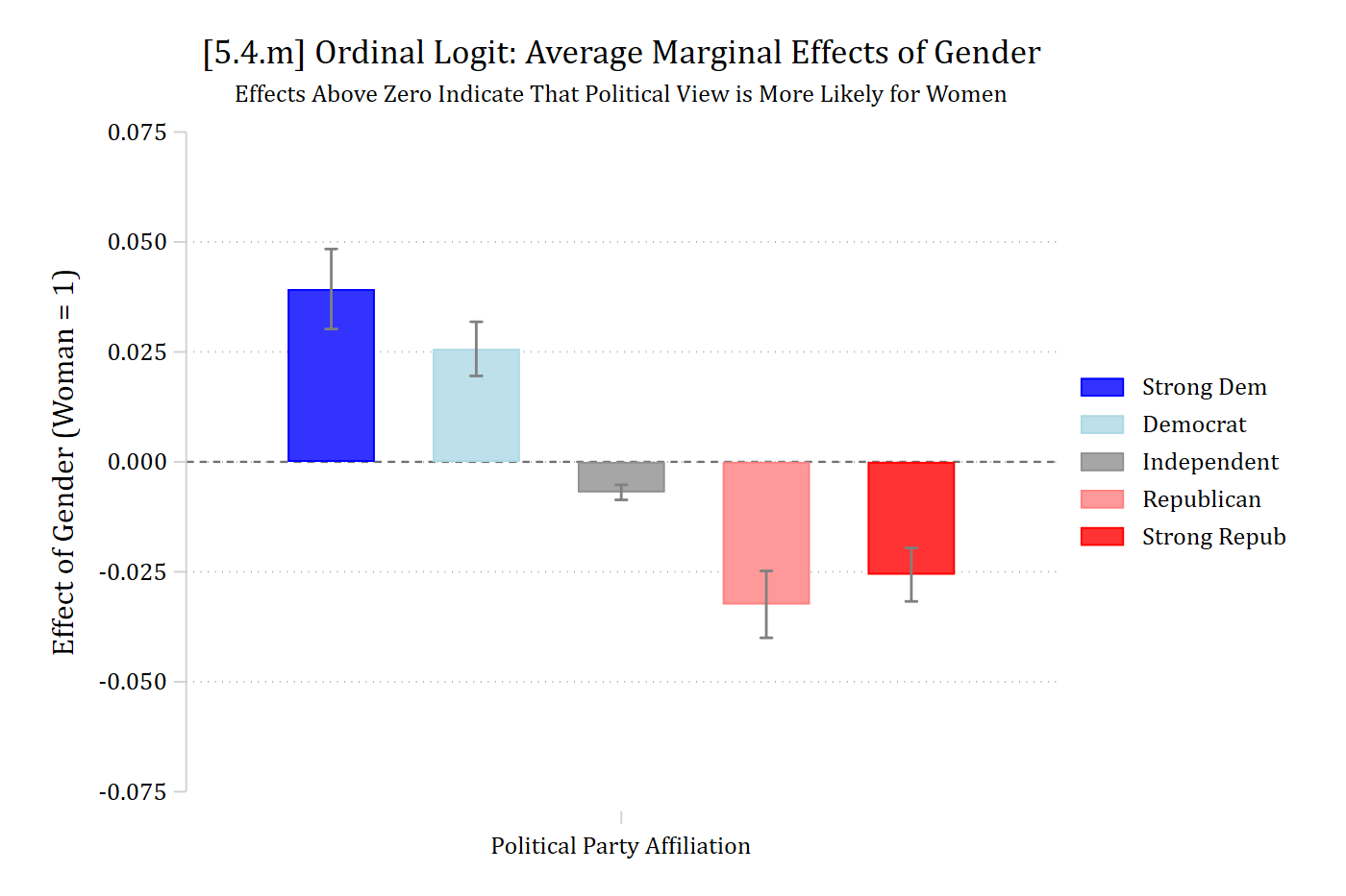
    • Gender has a significant effect on the probability of identifying with each of the five political party affiliations
*5.4.i
qui margins, at(age=(18(5)93))
marginsplot, noci ylab(0(.1).4) xlab(20(10)90) ///
    legend(order(1 "Strong Dem" 2 "Democrat" 3 "Independent" ///
        4 " Republican" 5 "Strong Repub")) ///
    plot1opts(lcolor(blue) lpat(solid)) ///
    plot2opts(lcolor(ltblue) lpat(dash)) ///
    plot3opts(lcolor(gs9) lpat(solid)) ///
    plot4opts(lcolor(red*.5) lpat(dash)) ///
    plot5opts(lcolor(red) lpat(solid)) ///
    plotopts(msym(none) lwidth(medthick)) ///
    xtitle("Age in Years") ytitle("Pr(Party Affiliation)") ///
    title("[5.4.i] Ordinal Logit: Predicted Probabilities of Political Party A
ffiliation")
Variables that uniquely identify margins: age
*5.4.k
qui margins, at(age=(-30000(1000)30000))
marginsplot, noci ylab(0(.2)1) xlab(-30000(10000)30000) ///
    legend(order(1 "Strong Dem" 2 "Democrat" 3 "Independent" ///
        4 " Republican" 5 "Strong Repub")) ///
    plot1opts(lcolor(blue) lpat(solid)) ///
    plot2opts(lcolor(ltblue) lpat(dash)) ///
    plot3opts(lcolor(gs9) lpat(solid)) ///
    plot4opts(lcolor(red*.5) lpat(dash)) ///
    plot5opts(lcolor(red) lpat(solid)) ///
    plotopts(msym(none) lwidth(medthick)) ///
    xtitle("Age in Years") ytitle("Pr(Party Affiliation)") ///
    title("[5.4.k] Ordinal Logit: Predicted Probabilities of Political Party A
ffiliation")
Variables that uniquely identify margins: age
*5.4.m
est restore oparty
(results oparty are active now)
qui margins, dydx(woman) predict(outcome(0)) post
est store ome0
est restore oparty
(results oparty are active now)
qui margins, dydx(woman) predict(outcome(1)) post
est store ome1
est restore oparty
(results oparty are active now)
qui margins, dydx(woman) predict(outcome(2)) post
est store ome2
est restore oparty
(results oparty are active now)
qui margins, dydx(woman) predict(outcome(3)) post
est store ome3
est restore oparty
(results oparty are active now)
qui margins, dydx(woman) predict(outcome(4)) post
est store ome4
coefplot (ome0, color(blue)) (ome1, color(ltblue)) (ome2, color(gs9)) ///
    (ome3, color(red*.5)) (ome4, color(red)), ///
    recast(bar) barw(0.1) vertical yline(0) ylab(-.075(.025).075, format(%4.3f
)) ///
    ciopts(recast(rcap) color(gs8)) citop ///
    legend(order(1 "Strong Dem" 3 "Democrat" 5 "Independent" ///
        7 "Republican" 9 "Strong Repub")) ///
    ytitle("Effect of Gender (Woman = 1)") xlab(1 "Political Party Affiliation
") ///
    title("[5.4.m] Ordinal Logit: Average Marginal Effects of Gender") ///
    subtitle("Effects Above Zero Indicate That Political View is More Likely f
or Women", size(small))

[5.4.i] Ordinal logit predicted probabilities of each party affiliation by age from 18 to 93: all five lines are flat (Democrat about 0.30, Republican about 0.22, Strong Dem and Independent about 0.18, Strong Repub about 0.11).

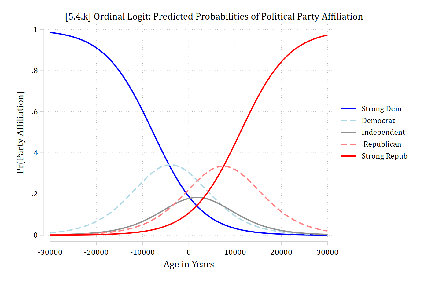
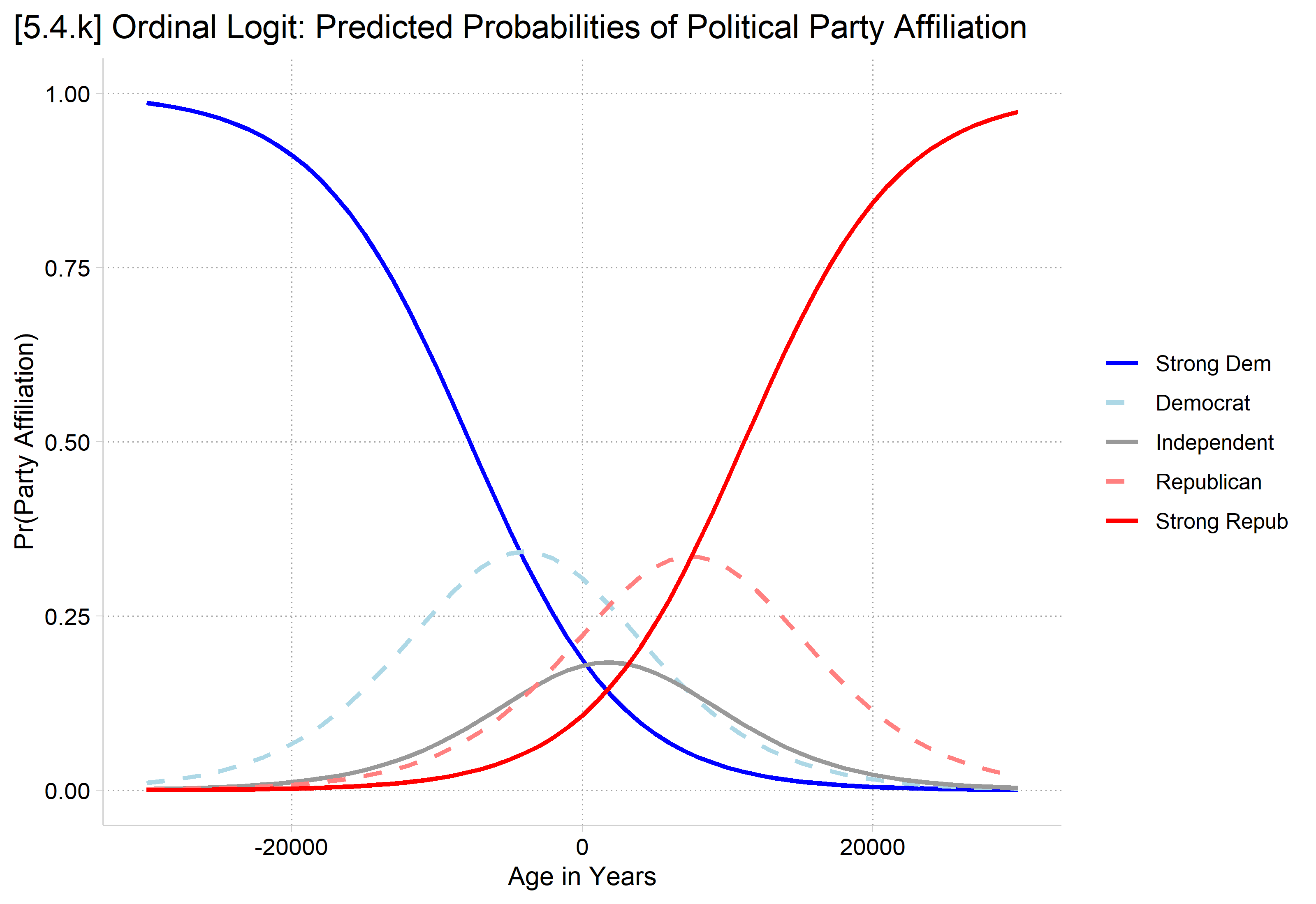
[5.4.k] Ordinal logit predicted probabilities of each party affiliation for impossible ages from -30,000 to 30,000: Pr(Strong Dem) falls from near 1 to near 0 and Pr(Strong Repub) rises from near 0 to near 1, with the middle categories peaking in between, which shows the ordinal functional form.

[5.4.m] Bar chart of the ordinal logit average marginal effects of gender (woman = 1) on each party affiliation: about 0.04 for Strong Dem, 0.03 for Democrat, -0.01 for Independent, -0.03 for Republican, and -0.03 for Strong Repub.

# Colors and line types for the party affiliation categories
party_colors <- c("blue", "lightblue", "gray60", "#FF8080", "red")
party_lines <- c("solid", "dashed", "solid", "dashed", "solid")

party_plot <- function(model, ages, title, ylimits = c(0, .4)) {
  pr <- avg_predictions(model, by = c("age", "group"),
    newdata = datagrid(age = ages, grid_type = "counterfactual"))
  ggplot(pr, aes(x = age, y = estimate, color = group, linetype = group)) +
    geom_line(linewidth = 1) +
    scale_color_manual(values = party_colors) +
    scale_linetype_manual(values = party_lines) +
    scale_y_continuous(limits = ylimits) +
    labs(title = title, x = "Age in Years", y = "Pr(Party Affiliation)",
      color = NULL, linetype = NULL) +
    theme(plot.title.position = "plot")
}

# 5.4.i
party_plot(oparty, seq(18, 93, 5),
  "[5.4.i] Ordinal Logit: Predicted Probabilities of Political Party Affiliation")

[5.4.i] Ordinal logit predicted probabilities of each party affiliation by age from 18 to 93: all five lines are flat (Democrat about 0.30, Republican about 0.22, Strong Dem and Independent about 0.18, Strong Repub about 0.11).

# 5.4.k
party_plot(oparty, seq(-30000, 30000, 1000),
  "[5.4.k] Ordinal Logit: Predicted Probabilities of Political Party Affiliation", c(0, 1))

[5.4.k] Ordinal logit predicted probabilities of each party affiliation for impossible ages from -30,000 to 30,000: Pr(Strong Dem) falls from near 1 to near 0 and Pr(Strong Repub) rises from near 0 to near 1, with the middle categories peaking in between, which shows the ordinal functional form.

# 5.4.m
me_party_plot <- function(model, title) {
  ggplot(avg_comparisons(model, variables = "woman"),
    aes(x = group, y = estimate, fill = group)) +
    geom_col(width = .7) +
    geom_errorbar(aes(ymin = conf.low, ymax = conf.high), width = .1, color = "gray40") +
    geom_hline(yintercept = 0, linetype = "dashed") +
    scale_fill_manual(values = party_colors) +
    scale_y_continuous(breaks = round(seq(-.075, .075, .025), 3), limits = c(-.075, .075)) +
    labs(title = title,
      subtitle = "Effects Above Zero Indicate That Political View is More Likely for Women",
      x = "Political Party Affiliation", y = "Effect of Gender (Woman = 1)", fill = NULL) +
    theme(plot.title.position = "plot", axis.text.x = element_blank())
}

me_party_plot(oparty, "[5.4.m] Ordinal Logit: Average Marginal Effects of Gender")

[5.4.m] Bar chart of the ordinal logit average marginal effects of gender (woman = 1) on each party affiliation: about 0.04 for Strong Dem, 0.03 for Democrat, -0.01 for Independent, -0.03 for Republican, and -0.03 for Strong Repub.

Brant test of parallel regressions

est restore oparty
(results oparty are active now)
brant
Brant test of parallel regression assumption

              |       chi2     p>chi2      df
 -------------+------------------------------
          All |    1218.28      0.000      45
 -------------+------------------------------
          age |     439.88      0.000       3
      1.woman |      14.15      0.003       3
        edyrs |     173.53      0.000       3
     1.parent |      33.37      0.000       3
    1.married |       7.82      0.050       3
       faminc |      66.82      0.000       3
   1.employed |       0.17      0.982       3
    2.region4 |      18.12      0.000       3
    3.region4 |      27.80      0.000       3
    4.region4 |       0.72      0.868       3
    2012.year |       6.58      0.086       3
    2014.year |       8.18      0.042       3
    2016.year |       1.64      0.650       3
    2018.year |       2.48      0.479       3
    2021.year |      58.38      0.000       3

A significant test statistic provides evidence that the parallel
regression assumption has been violated.
brant(oparty)
-------------------------------------------- 
Test for    X2  df  probability 
-------------------------------------------- 
Omnibus     1233.04 45  0
age     439.88  3   0
womanWomen  14.15   3   0
edyrs       173.53  3   0
parentParent    33.37   3   0
marriedMarried  7.82    3   0.05
faminc      66.82   3   0
employedYes 0.17    3   0.98
region4Midwest  18.12   3   0
region4South    27.8    3   0
region4West 0.72    3   0.87
year2012    6.58    3   0.09
year2014    8.18    3   0.04
year2016    1.64    3   0.65
year2018    2.48    3   0.48
year2021    58.38   3   0
-------------------------------------------- 

H0: Parallel Regression Assumption holds

A Brant test indicates that the model violates the parallel regression assumption of the ordinal logit model (p < 0.001). Both focal variables of age and gender have relationships with political party affiliation that are not strictly ordered in nature.

Multinomial logit model for political party affiliation

///////////////////////
// Multinomial Logit //
///////////////////////
qui mlogit partyid5 c.age i.woman c.edyrs i.parent i.married ///
    c.faminc i.employed i.region4 i.year
est store mparty
mlogtest
Wald tests for independent variables (N=13430)

  Ho: All coefficients associated with given variable(s) are 0

                 |      chi2    df   P>chi2
-----------------+-------------------------
             age |   423.542     4    0.000
         1.woman |    79.101     4    0.000
           edyrs |   232.132     4    0.000
        1.parent |    39.427     4    0.000
       1.married |   126.498     4    0.000
          faminc |    88.130     4    0.000
      1.employed |     9.855     4    0.043
       2.region4 |    43.675     4    0.000
       3.region4 |    71.695     4    0.000
       4.region4 |     9.170     4    0.057
       2012.year |     7.911     4    0.095
       2014.year |     8.189     4    0.085
       2016.year |     1.920     4    0.750
       2018.year |     4.913     4    0.296
       2021.year |    61.137     4    0.000
# Multinomial Logit
mparty <- multinom(partyid5 ~ age + woman + edyrs + parent + married + faminc +
  employed + region4 + year, data = party, Hess = TRUE, trace = FALSE)

# Likelihood-ratio tests (region4 and year are each tested as one variable)
Anova(mparty, type = 2)
Analysis of Deviance Table (Type II tests)

Response: partyid5
         LR Chisq Df Pr(>Chisq)    
age        443.76  4  < 2.2e-16 ***
woman       79.63  4  < 2.2e-16 ***
edyrs      238.87  4  < 2.2e-16 ***
parent      40.09  4  4.148e-08 ***
married    127.69  4  < 2.2e-16 ***
faminc      91.38  4  < 2.2e-16 ***
employed     9.85  4    0.04299 *  
region4    103.88 12  < 2.2e-16 ***
year       119.14 20  4.107e-16 ***
---
Signif. codes:  0 '***' 0.001 '**' 0.01 '*' 0.05 '.' 0.1 ' ' 1
  • In terms of the coefficients:
    • Age has a significant effect
    • Gender has a significant effect
mchange age woman, amount(sd)
mlogit: Changes in Pr(y) | Number of obs = 13430

Expression: Pr(partyid5), predict(outcome())

              | Strong ~m   Democrat  Indepen~t  Republi~n  Strong ~b 
--------------+------------------------------------------------------
age           |                                                      
          +SD |     0.041     -0.038     -0.047     -0.000      0.043 
      p-value |     0.000      0.000      0.000      0.941      0.000 
woman         |                                                      
 Women vs Men |     0.047      0.013      0.001     -0.049     -0.012 
      p-value |     0.000      0.115      0.869      0.000      0.030 

Average predictions

             | Strong ~m   Democrat  Indepen~t  Republi~n  Strong ~b 
-------------+------------------------------------------------------
  Pr(y|base) |     0.186      0.304      0.179      0.223      0.108 
# AMEs (mchange's +SD change starts at each observation's value)
avg_comparisons(mparty, variables = list(age = sd(party$age)))

        Group  Estimate Std. Error        z Pr(>|z|)     S    2.5 %   97.5 %
 Strong Dem    0.041237    0.00427   9.6572   <0.001  70.9  0.03287  0.04961
 Democrat     -0.037511    0.00410  -9.1400   <0.001  63.8 -0.04556 -0.02947
 Independent  -0.046613    0.00291 -15.9934   <0.001 188.8 -0.05233 -0.04090
 Republican   -0.000304    0.00412  -0.0737    0.941   0.1 -0.00838  0.00777
 Strong Repub  0.043191    0.00414  10.4291   <0.001  82.2  0.03507  0.05131

Term: age
Type: probs
Comparison: +17.2933969697999
avg_comparisons(mparty, variables = "woman")

        Group Estimate Std. Error      z Pr(>|z|)    S   2.5 %   97.5 %
 Strong Dem     0.0467    0.00671  6.955   <0.001 38.0  0.0335  0.05981
 Democrat       0.0127    0.00806  1.576   0.1150  3.1 -0.0031  0.02852
 Independent    0.0011    0.00667  0.165   0.8686  0.2 -0.0120  0.01418
 Republican    -0.0487    0.00735 -6.629   <0.001 34.8 -0.0632 -0.03433
 Strong Repub  -0.0117    0.00540 -2.172   0.0298  5.1 -0.0223 -0.00115

Term: woman
Type: probs
Comparison: Women - Men
  • In terms of AMEs:
    • Age has an effect on the probability of identifying with four of the five political party affiliations
    • Gender has a significant effect on the probability of identifying with three of the five political party affiliations
*5.4.n
qui margins, at(age=(18(5)93))
marginsplot, noci ylab(0(.1).4) xlab(20(10)90) ///
    legend(order(1 "Strong Dem" 2 "Democrat" 3 "Independent" ///
        4 " Republican" 5 "Strong Repub")) ///
    plot1opts(lcolor(blue) lpat(solid)) ///
    plot2opts(lcolor(ltblue) lpat(dash)) ///
    plot3opts(lcolor(gs9) lpat(solid)) ///
    plot4opts(lcolor(red*.5) lpat(dash)) ///
    plot5opts(lcolor(red) lpat(solid)) ///
    plotopts(msym(none) lwidth(medthick)) ///
    xtitle("Age in Years") ytitle("Pr(Party Affiliation)") ///
    title("[5.4.n] Multinomial Logit: Predicted Probabilities of Political Par
ty Affiliation")
Variables that uniquely identify margins: age
*5.4.o
qui margins, at(age=(-500(10)500))
marginsplot, noci ylab(0(.2)1) xlab(-500(100)500) ///
    legend(order(1 "Strong Dem" 2 "Democrat" 3 "Independent" ///
        4 " Republican" 5 "Strong Repub")) ///
    plot1opts(lcolor(blue) lpat(solid)) ///
    plot2opts(lcolor(ltblue) lpat(dash)) ///
    plot3opts(lcolor(gs9) lpat(solid)) ///
    plot4opts(lcolor(red*.5) lpat(dash)) ///
    plot5opts(lcolor(red) lpat(solid)) ///
    plotopts(msym(none) lwidth(medthick)) ///
    xtitle("Age in Years") ytitle("Pr(Party Affiliation)") ///
    title("[5.4.o] Multinomial Logit: Predicted Probabilities of Political Par
ty Affiliation")
Variables that uniquely identify margins: age

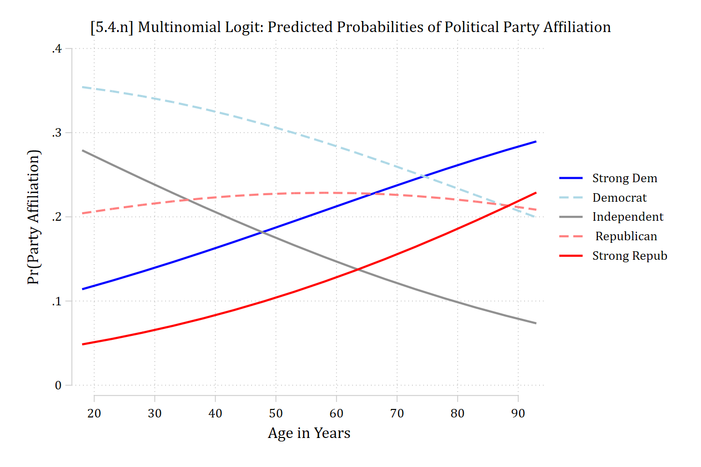
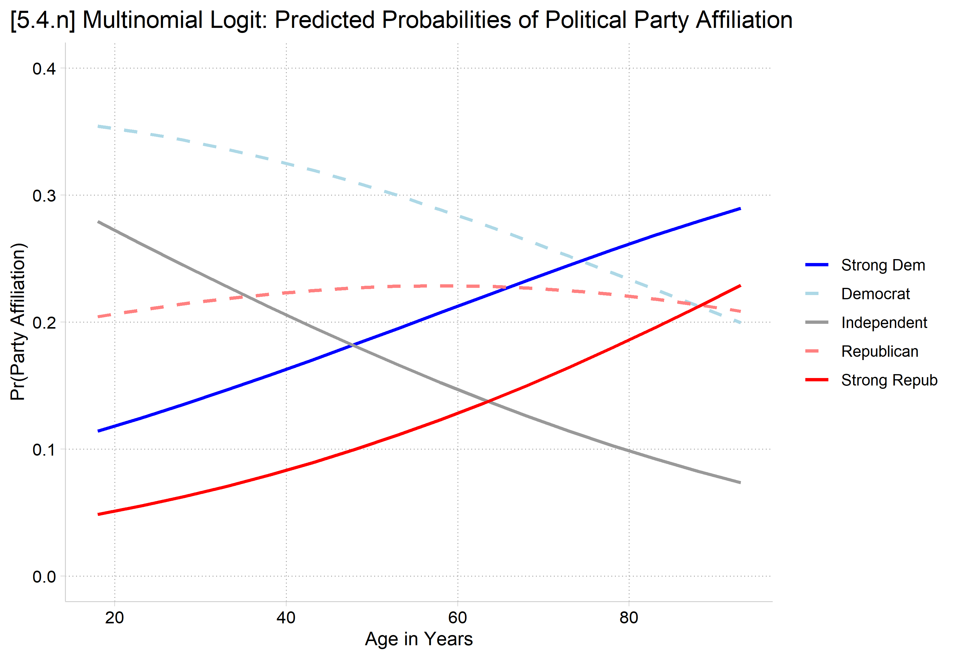
[5.4.n] Multinomial logit predicted probabilities of each party affiliation by age from 18 to 93: Strong Dem and Strong Repub rise with age (about 0.11 to 0.29 and 0.05 to 0.23), Democrat and Independent fall (about 0.35 to 0.20 and 0.28 to 0.07), and Republican stays near 0.21.

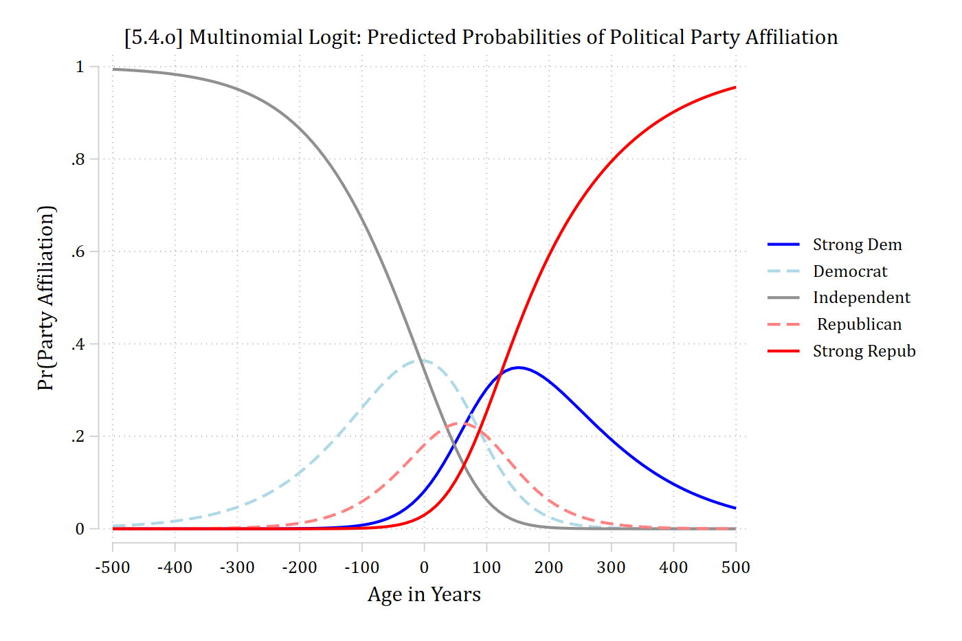
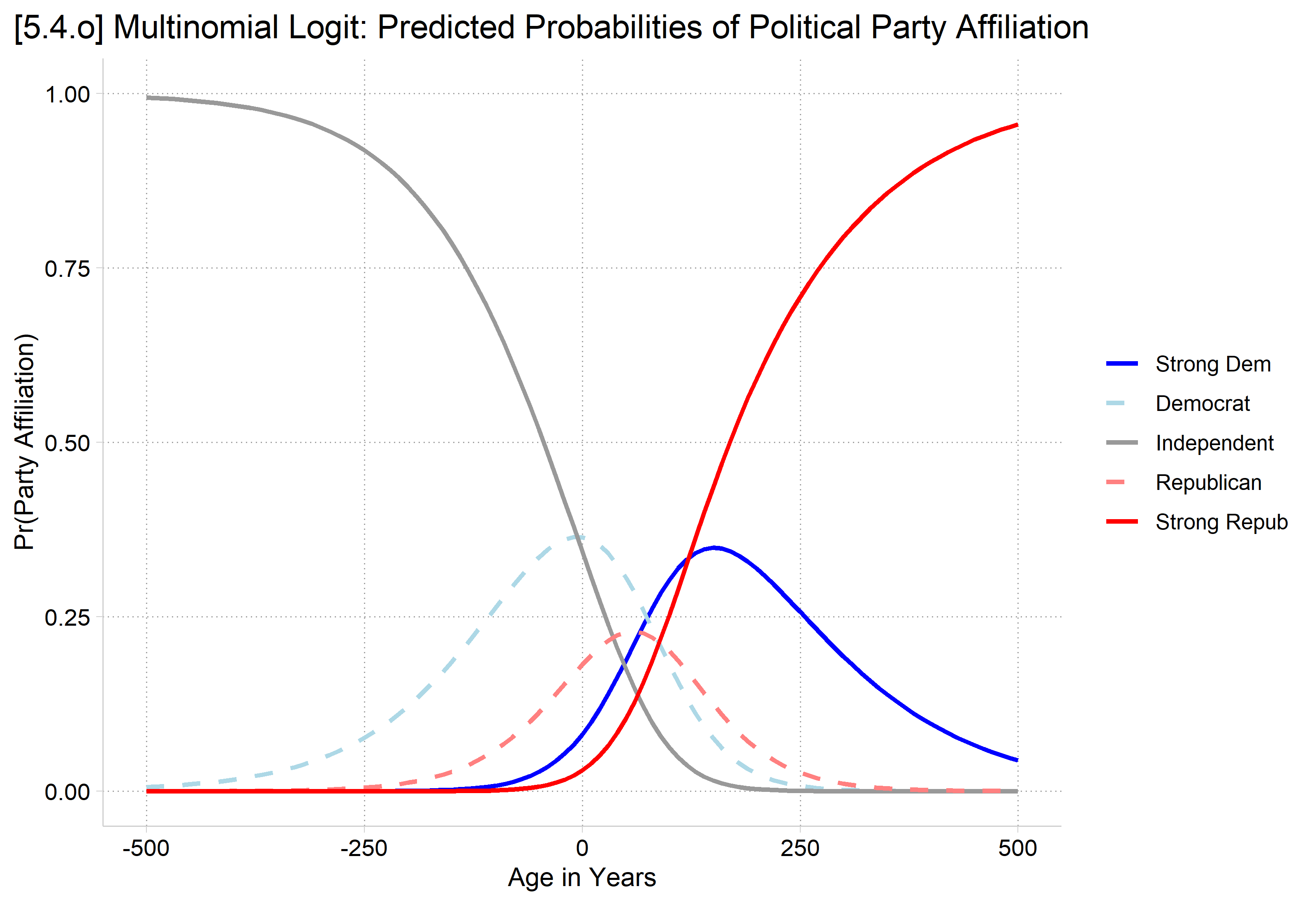
[5.4.o] Multinomial logit predicted probabilities of each party affiliation for impossible ages from -500 to 500: Independent dominates at very negative ages and Strong Repub at very high ages, a pattern that does not follow the ordering of the categories.

# 5.4.n
party_plot(mparty, seq(18, 93, 5),
  "[5.4.n] Multinomial Logit: Predicted Probabilities of Political Party Affiliation")

[5.4.n] Multinomial logit predicted probabilities of each party affiliation by age from 18 to 93: Strong Dem and Strong Repub rise with age (about 0.11 to 0.29 and 0.05 to 0.23), Democrat and Independent fall (about 0.35 to 0.20 and 0.28 to 0.07), and Republican stays near 0.21.

# 5.4.o
party_plot(mparty, seq(-500, 500, 10),
  "[5.4.o] Multinomial Logit: Predicted Probabilities of Political Party Affiliation", c(0, 1))

[5.4.o] Multinomial logit predicted probabilities of each party affiliation for impossible ages from -500 to 500: Independent dominates at very negative ages and Strong Repub at very high ages, a pattern that does not follow the ordering of the categories.

*AMEs of gender from mlogit (for the comparison graph below)
est restore mparty
(results mparty are active now)
qui margins, dydx(woman) predict(outcome(0)) post
est store me0
est restore mparty
(results mparty are active now)
qui margins, dydx(woman) predict(outcome(1)) post
est store me1
est restore mparty
(results mparty are active now)
qui margins, dydx(woman) predict(outcome(2)) post
est store me2
est restore mparty
(results mparty are active now)
qui margins, dydx(woman) predict(outcome(3)) post
est store me3
est restore mparty
(results mparty are active now)
qui margins, dydx(woman) predict(outcome(4)) post
est store me4
// Make graphs that can combine nicely for comparison
est restore oparty
(results oparty are active now)
qui margins, at(age=(18(5)93))
marginsplot, noci ylab(0(.1).4) xlab(20(10)90) ///
    legend(order(1 "Strong Dem" 2 "Democrat" 3 "Independent" ///
        4 " Republican" 5 "Strong Repub") position(6) rows(3)) ///
    plot1opts(lcolor(blue) lpat(solid)) ///
    plot2opts(lcolor(ltblue*1.2) lpat(dash)) ///
    plot3opts(lcolor(gs9) lpat(solid)) ///
    plot4opts(lcolor(red*.7) lpat(dash)) ///
    plot5opts(lcolor(red) lpat(solid)) ///
    plotopts(msym(none) lwidth(medthick)) ///
    xtitle("Age in Years") ytitle("Pr(Party Affiliation)") ///
    title("Ordinal Logit", size(large)) saving(oage.gph, replace)
Variables that uniquely identify margins: age
(file oage.gph not found)
file oage.gph saved
est restore mparty
(results mparty are active now)
qui margins, at(age=(18(5)93))
marginsplot, noci ylab(0(.1).4) xlab(20(10)90) ///
    legend(order(1 "Strong Dem" 2 "Democrat" 3 "Independent" ///
        4 " Republican" 5 "Strong Repub") position(6) rows(3)) ///
    plot1opts(lcolor(blue) lpat(solid)) ///
    plot2opts(lcolor(ltblue*1.2) lpat(dash)) ///
    plot3opts(lcolor(gs9) lpat(solid)) ///
    plot4opts(lcolor(red*.7) lpat(dash)) ///
    plot5opts(lcolor(red) lpat(solid)) ///
    plotopts(msym(none) lwidth(medthick)) ///
    xtitle("Age in Years") ytitle("Pr(Party Affiliation)") ///
    title("Multinomial Logit", size(large)) saving(mage.gph, replace)
Variables that uniquely identify margins: age
(file mage.gph not found)
file mage.gph saved
graph combine oage.gph mage.gph
coefplot (ome0, color(blue)) (ome1, color(ltblue)) (ome2, color(gs9)) ///
    (ome3, color(red*.5)) (ome4, color(red)), ///
    recast(bar) barw(0.1) vertical yline(0) ylab(-.075(.025).075, format(%4.3f
)) ///
    ciopts(recast(rcap) color(gs8)) citop ///
    legend(order(1 "Strong Dem" 3 "Democrat" 5 "Independent" ///
        7 "Republican" 9 "Strong Repub") position(6) rows(3)) ///
    ytitle("Effect of Gender (Woman = 1)") xlab(1 "Political Party Affiliation
") ///
    title("Ordinal Logit", size(large)) saving(ome.gph, replace)
(file ome.gph not found)
file ome.gph saved
coefplot (me0, color(blue)) (me1, color(ltblue)) (me2, color(gs9)) ///
    (me3, color(red*.5)) (me4, color(red)), ///
    recast(bar) barw(0.1) vertical yline(0) ylab(-.075(.025).075, format(%4.3f
)) ///
    ciopts(recast(rcap) color(gs8)) citop ///
    legend(order(1 "Strong Dem" 3 "Democrat" 5 "Independent" ///
        7 "Republican" 9 "Strong Repub") position(6) rows(3)) ///
    ytitle("Effect of Gender (Woman = 1)") xlab(1 "Political Party Affiliation
") ///
    title("Multinomial Logit", size(large)) saving(mme.gph, replace)
(file mme.gph not found)
file mme.gph saved
graph combine ome.gph mme.gph

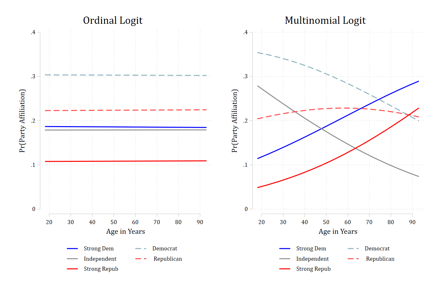
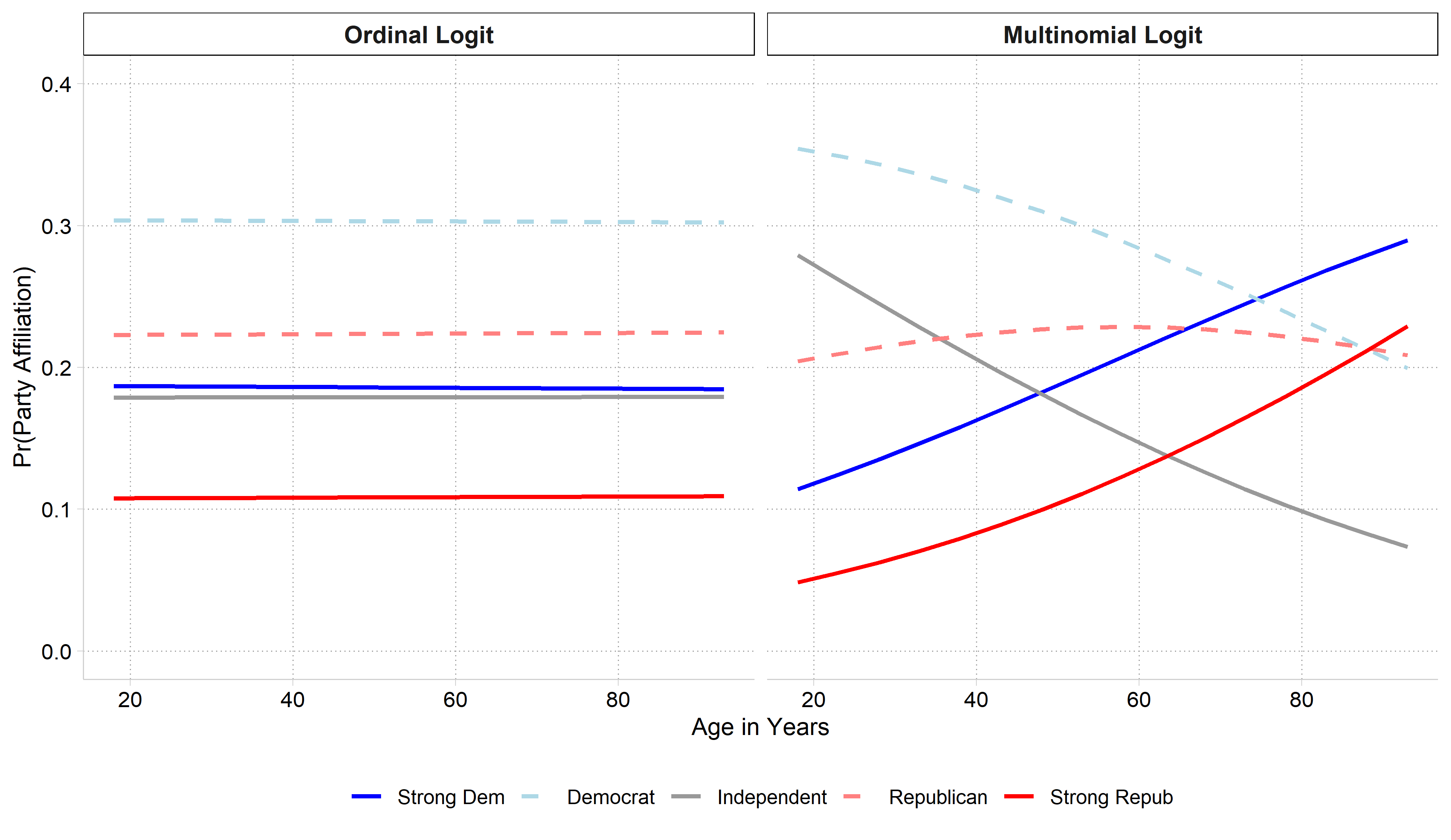
Ordinal logit and multinomial logit predicted probabilities of party affiliation by age side by side: the ordinal model's lines are flat, while the multinomial model shows Strong Dem and Strong Repub rising and Democrat and Independent falling with age.

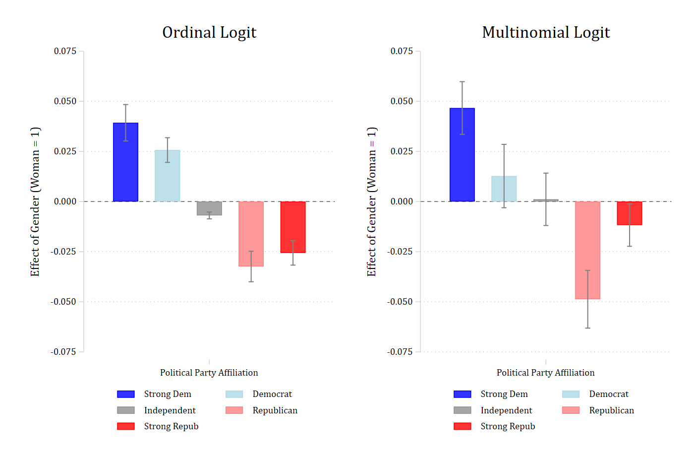
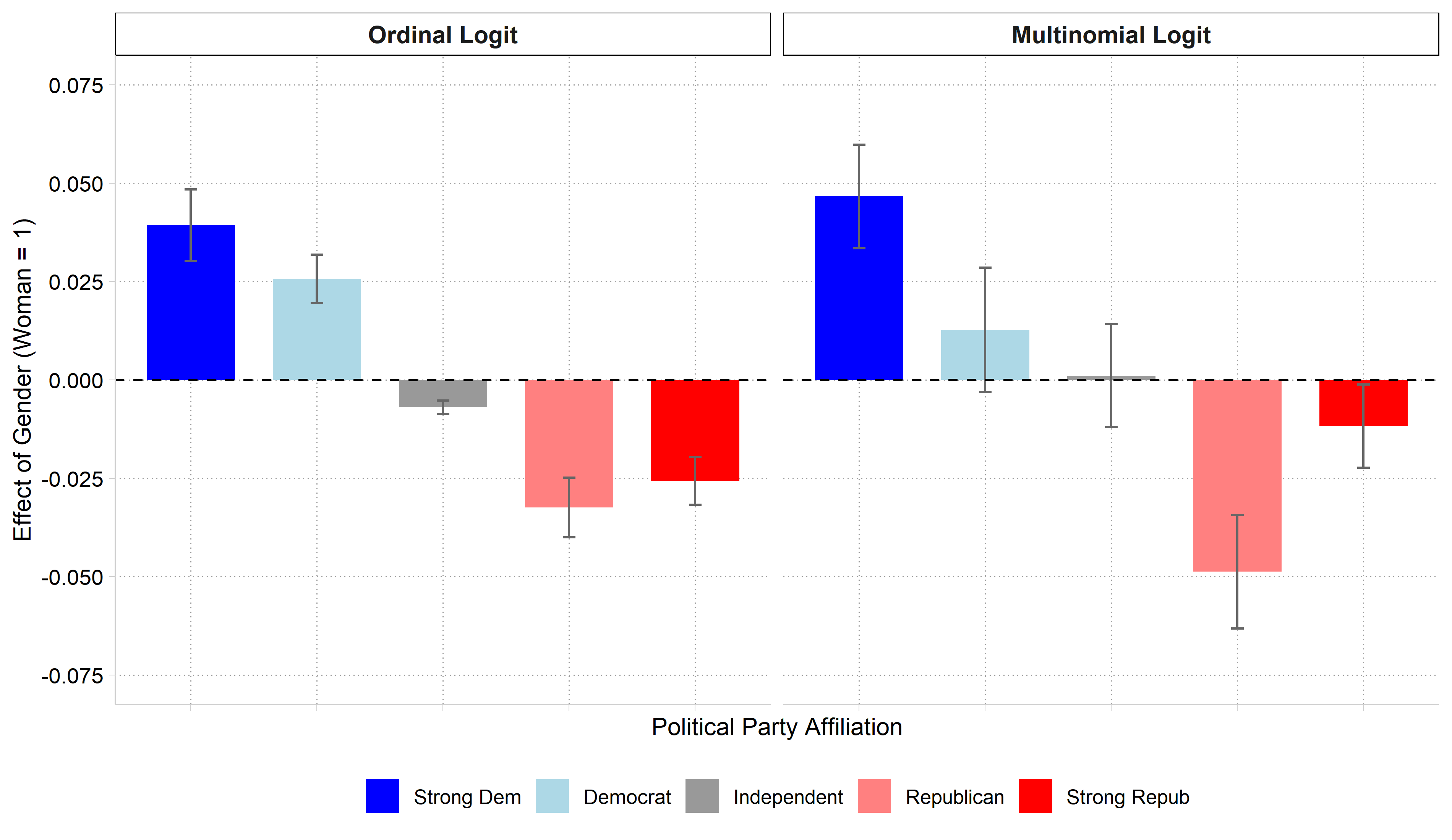
Ordinal logit and multinomial logit average marginal effects of gender side by side: the ordinal model has effects that shift steadily from positive for Strong Dem to negative for Strong Repub, while the multinomial model's largest effects are for Strong Dem (positive) and Republican (negative), with Strong Repub only slightly negative.

# Predictions from both models side by side
pr_party <- bind_rows(
  "Ordinal Logit" = avg_predictions(oparty, by = c("age", "group"),
    newdata = datagrid(age = seq(18, 93, 5), grid_type = "counterfactual")),
  "Multinomial Logit" = avg_predictions(mparty, by = c("age", "group"),
    newdata = datagrid(age = seq(18, 93, 5), grid_type = "counterfactual")),
  .id = "model") |>
  mutate(model = factor(model, levels = c("Ordinal Logit", "Multinomial Logit")))

ggplot(pr_party, aes(x = age, y = estimate, color = group, linetype = group)) +
  geom_line(linewidth = 1) +
  facet_wrap(~ model) +
  scale_color_manual(values = party_colors) +
  scale_linetype_manual(values = party_lines) +
  scale_y_continuous(limits = c(0, .4)) +
  labs(x = "Age in Years", y = "Pr(Party Affiliation)", color = NULL, linetype = NULL) +
  theme(legend.position = "bottom")

Ordinal logit and multinomial logit predicted probabilities of party affiliation by age side by side: the ordinal model's lines are flat, while the multinomial model shows Strong Dem and Strong Repub rising and Democrat and Independent falling with age.

# AMEs of gender from both models side by side
me_party <- bind_rows(
  "Ordinal Logit" = avg_comparisons(oparty, variables = "woman"),
  "Multinomial Logit" = avg_comparisons(mparty, variables = "woman"),
  .id = "model") |>
  mutate(model = factor(model, levels = c("Ordinal Logit", "Multinomial Logit")))

ggplot(me_party, aes(x = group, y = estimate, fill = group)) +
  geom_col(width = .7) +
  geom_errorbar(aes(ymin = conf.low, ymax = conf.high), width = .1, color = "gray40") +
  geom_hline(yintercept = 0, linetype = "dashed") +
  facet_wrap(~ model) +
  scale_fill_manual(values = party_colors) +
  scale_y_continuous(breaks = round(seq(-.075, .075, .025), 3), limits = c(-.075, .075)) +
  labs(x = "Political Party Affiliation", y = "Effect of Gender (Woman = 1)", fill = NULL) +
  theme(legend.position = "bottom", axis.text.x = element_blank())

Ordinal logit and multinomial logit average marginal effects of gender side by side: the ordinal model has effects that shift steadily from positive for Strong Dem to negative for Strong Repub, while the multinomial model's largest effects are for Strong Dem (positive) and Republican (negative), with Strong Repub only slightly negative.

// 5.4.r - Compare predictions for individual obs
est restore mparty
(results mparty are active now)
predict mpr1 mpr2 mpr3 mpr4 mpr5
(option pr assumed; predicted probabilities)
est restore oparty
(results oparty are active now)
predict opr1 opr2 opr3 opr4 opr5
(option pr assumed; predicted probabilities)
scatter mpr1 opr1, jitter(2) xlab(0(.1).4) ylab(0(.1).5) mcol(blue) ///
    xtitle("Pr(Strong Dem) from Ordinal Logit") ytitle("Pr(Strong Dem) Multino
mial Logit") ///
    msize(vsmall) saving(pr1.gph, replace)
file pr1.gph saved
scatter mpr2 opr2, jitter(2) xlab(0(.1).4) ylab(0(.1).5) mcol(ltblue) ///
    xtitle("Pr(Democrat) from Ordinal Logit") ytitle("Pr(Democrat) Multinomial
 Logit") ///
    msize(vsmall) saving(pr2.gph, replace)
file pr2.gph saved
scatter mpr4 opr4, jitter(2) xlab(0(.1).4) ylab(0(.1).5) mcol(red*.5) ///
    xtitle("Pr(Republican) from Ordinal Logit") ytitle("Pr(Republican) Multino
mial Logit") ///
    msize(vsmall) saving(pr4.gph, replace)
file pr4.gph saved
scatter mpr5 opr5, jitter(2) xlab(0(.1).4) ylab(0(.1).5) mcol(red) ///
    xtitle("Pr(Strong Rep) from Ordinal Logit") ytitle("Pr(Strong Rep) Multino
mial Logit") ///
    msize(vsmall) saving(pr5.gph, replace)
(file pr5.gph not found)
file pr5.gph saved
graph combine pr1.gph pr2.gph pr4.gph pr5.gph, ///
    title("[5.4.r] Predicted Probabilities from Multinomial Logit (y-axis)" //
/
        "vs Ordinal Logit (x-axis)", size(medsmall))
*5.4.s
scatter mpr3 opr3, jitter(2) xlab(0(.1).4) ylab(0(.1).7) mcol(gs9) ///
    xtitle("Pr(Independent) from Ordinal Logit") ytitle("Pr(Independent) Multi
nomial Logit") ///
    title("[5.4.s] Predicted Probabilities from Multinomial Logit (y-axis)" //
/
        "vs Ordinal Logit (x-axis)", size(medsmall)) msize(vsmall)

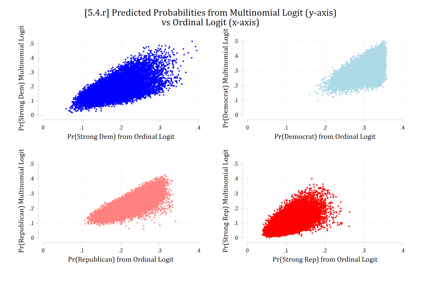
[5.4.r] Four scatterplots of each observation's predicted probability of Strong Dem, Democrat, Republican, and Strong Rep from the multinomial logit (y-axis) against the ordinal logit (x-axis): the points form wide clouds rather than lines, so the two models often disagree for individual people.

[5.4.s] Scatterplot of each observation's predicted probability of Independent from the multinomial logit (y-axis, about 0.03 to 0.7) against the ordinal logit (x-axis, about 0.14 to 0.19): the ordinal model gives nearly everyone the same probability while the multinomial model's predictions vary widely.

# 5.4.r - Compare predictions for individual obs
pr_party_obs <- data.frame(outcome = rep(levels(party$partyid5), each = nrow(party)),
  multinomial = as.vector(predict(mparty, type = "probs")),
  ordinal = as.vector(predict(oparty, type = "probs"))) |>
  mutate(outcome = factor(outcome, levels = levels(party$partyid5)))

ggplot(filter(pr_party_obs, outcome != "Independent"),
  aes(x = ordinal, y = multinomial, color = outcome)) +
  geom_point(size = .3, alpha = .3) +
  facet_wrap(~ outcome) +
  scale_color_manual(values = party_colors[-3]) +
  scale_x_continuous(breaks = seq(0, .4, .1), limits = c(0, .4)) +
  scale_y_continuous(breaks = seq(0, .5, .1), limits = c(0, .5)) +
  labs(title = "[5.4.r] Predicted Probabilities from Multinomial Logit (y-axis) vs Ordinal Logit (x-axis)",
    x = "Pr from Ordinal Logit", y = "Pr from Multinomial Logit") +
  theme(plot.title.position = "plot", legend.position = "none")

[5.4.r] Four scatterplots of each observation's predicted probability of Strong Dem, Democrat, Republican, and Strong Rep from the multinomial logit (y-axis) against the ordinal logit (x-axis): the points form wide clouds rather than lines, so the two models often disagree for individual people.

# 5.4.s
ggplot(filter(pr_party_obs, outcome == "Independent"), aes(x = ordinal, y = multinomial)) +
  geom_point(size = .3, alpha = .3, color = "gray60") +
  scale_x_continuous(breaks = seq(0, .4, .1), limits = c(0, .4)) +
  scale_y_continuous(breaks = seq(0, .7, .1), limits = c(0, .7)) +
  labs(title = "[5.4.s] Predicted Probabilities from Multinomial Logit (y-axis) vs Ordinal Logit (x-axis)",
    x = "Pr(Independent) from Ordinal Logit", y = "Pr(Independent) Multinomial Logit") +
  theme(plot.title.position = "plot")

[5.4.s] Scatterplot of each observation's predicted probability of Independent from the multinomial logit (y-axis, about 0.03 to 0.7) against the ordinal logit (x-axis, about 0.14 to 0.19): the ordinal model gives nearly everyone the same probability while the multinomial model's predictions vary widely.

Testing predictions and effects across models

  • The comparisons of the ordinal and nominal model in this section are informal
    • I.e., I did not conduct any significance tests as to whether the predictions and/or MEs were different across the two models
  • Mize, Doan, and Long (2019) develop a method that can be used to test for differences across the ordinal and multinomial logit models (see example 6.5 in the article)
    • In Stata, the mecompare command automates these tests
    • In R, use suest to combine the two model’s estimates, and avg_comparisons to calculate the MEs to compare
*mecompare with two models() combines estimates using SUEST and calculates
**difference in MEs across models
mecompare age, models(oparty mparty) amount(sd)
mecompare uses vce(robust) for all models. Standard errors from mecompare will d
> iffer from the specified model(s) because vce(robust) was not used on at least
>  one of the models specified in the models( ) option. We strongly recommend re
> fitting the first (ologit) and second (mlogit) models with vce(robust). See vc
> e_option for details on vce(robust).

Predicting: Pr(partyid5)
Marginal effects and cross-model differences (N_oparty=13430) (N_mparty=13430)

                                 |  ME #   Estimate  Robust SE      P>|z|
---------------------------------+---------------------------------------
age + SD (centered)              |                                       
             Strong Dem - oparty |     1     -0.000      0.003      0.851
             Strong Dem - mparty |     2      0.041      0.004      0.000
         Strong Dem - Difference |     3     -0.041      0.003      0.000
               Democrat - oparty |     4     -0.000      0.002      0.851
               Democrat - mparty |     5     -0.034      0.004      0.000
           Democrat - Difference |     6      0.033      0.004      0.000
            Independent - oparty |     7      0.000      0.000      0.850
            Independent - mparty |     8     -0.050      0.004      0.000
        Independent - Difference |     9      0.050      0.004      0.000
             Republican - oparty |    10      0.000      0.002      0.851
             Republican - mparty |    11      0.004      0.004      0.301
         Republican - Difference |    12     -0.004      0.004      0.281
           Strong Repub - oparty |    13      0.000      0.002      0.851
           Strong Repub - mparty |    14      0.039      0.003      0.000
       Strong Repub - Difference |    15     -0.038      0.003      0.000
# Center changes in continuous IVs on each observation's value (as mecompare does)
options(marginaleffects_contrast_direction = "center")

# suest combines the estimates of the two models
party_suest <- suest(oparty, mparty, model_names = c("oparty", "mparty"))

me_age <- avg_comparisons(party_suest, variables = list(age = sd(party$age)),
  newdata = party)
me_age

                Group  Estimate Std. Error       z Pr(>|z|)     S     2.5 %   97.5 %
 oparty::Strong Dem   -5.00e-04   0.002651  -0.188    0.851   0.2 -0.005696  0.00470
 oparty::Democrat     -3.16e-04   0.001679  -0.188    0.851   0.2 -0.003607  0.00298
 oparty::Independent   8.97e-05   0.000475   0.189    0.850   0.2 -0.000842  0.00102
 oparty::Republican    4.05e-04   0.002151   0.188    0.851   0.2 -0.003811  0.00462
 oparty::Strong Repub  3.21e-04   0.001704   0.188    0.851   0.2 -0.003019  0.00366
 mparty::Strong Dem    4.10e-02   0.003621  11.317   <0.001  96.2  0.033884  0.04808
 mparty::Democrat     -3.37e-02   0.004434  -7.607   <0.001  45.0 -0.042418 -0.02504
 mparty::Independent  -5.02e-02   0.003675 -13.652   <0.001 138.6 -0.057381 -0.04297
 mparty::Republican    4.26e-03   0.004121   1.034    0.301   1.7 -0.003814  0.01234
 mparty::Strong Repub  3.87e-02   0.003172  12.187   <0.001 111.1  0.032443  0.04488

Term: age
Type: response
Comparison: +17.2933969697999
# Difference between the models for each outcome: oparty - mparty
model_diffs <- function(x) {
  data.frame(term = sub("^oparty::", "", x$group[1:5]),
    estimate = x$estimate[1:5] - x$estimate[6:10])
}
hypotheses(me_age, hypothesis = model_diffs)

         Term Estimate Std. Error      z Pr(>|z|)     S   2.5 %   97.5 %
 Strong Dem   -0.04148    0.00251 -16.55   <0.001 202.0 -0.0464 -0.03657
 Democrat      0.03341    0.00412   8.11   <0.001  50.8  0.0253  0.04149
 Independent   0.05027    0.00364  13.80   <0.001 141.5  0.0431  0.05741
 Republican   -0.00386    0.00358  -1.08    0.281   1.8 -0.0109  0.00315
 Strong Repub -0.03834    0.00267 -14.38   <0.001 153.4 -0.0436 -0.03312

The average marginal effect of age is significantly different across the ordinal and nominal model for the probability of identifying as a strong Democrat, a Democrat, an independent, and a strong Republican (all cross-model differences p < .001). The models suggest similar non-significant effects of age on the probability of identifying as a Republican (cross-model difference p = n.s.).

*binary IV woman
mecompare woman, models(oparty mparty)
mecompare uses vce(robust) for all models. Standard errors from mecompare will d
> iffer from the specified model(s) because vce(robust) was not used on at least
>  one of the models specified in the models( ) option. We strongly recommend re
> fitting the first (ologit) and second (mlogit) models with vce(robust). See vc
> e_option for details on vce(robust).

Predicting: Pr(partyid5)
Marginal effects and cross-model differences (N_oparty=13430) (N_mparty=13430)

                                 |  ME #   Estimate  Robust SE      P>|z|
---------------------------------+---------------------------------------
woman                            |                                       
                 Women - Men     |                                       
             Strong Dem - oparty |     1      0.039      0.005      0.000
             Strong Dem - mparty |     2      0.047      0.007      0.000
         Strong Dem - Difference |     3     -0.007      0.005      0.129
               Democrat - oparty |     4      0.026      0.003      0.000
               Democrat - mparty |     5      0.013      0.008      0.114
           Democrat - Difference |     6      0.013      0.007      0.080
            Independent - oparty |     7     -0.007      0.001      0.000
            Independent - mparty |     8      0.001      0.007      0.869
        Independent - Difference |     9     -0.008      0.007      0.228
             Republican - oparty |    10     -0.032      0.004      0.000
             Republican - mparty |    11     -0.049      0.007      0.000
         Republican - Difference |    12      0.016      0.006      0.009
           Strong Repub - oparty |    13     -0.026      0.003      0.000
           Strong Repub - mparty |    14     -0.012      0.005      0.031
       Strong Repub - Difference |    15     -0.014      0.005      0.002
# binary IV woman
me_woman <- avg_comparisons(party_suest, variables = "woman", newdata = party)
me_woman

                Group Estimate Std. Error      z Pr(>|z|)    S    2.5 %   97.5 %
 oparty::Strong Dem    0.03930   0.004676  8.403   <0.001 54.4  0.03013  0.04846
 oparty::Democrat      0.02569   0.003150  8.156   <0.001 51.4  0.01952  0.03187
 oparty::Independent  -0.00693   0.000884 -7.843   <0.001 47.7 -0.00867 -0.00520
 oparty::Republican   -0.03241   0.003917 -8.274   <0.001 52.8 -0.04009 -0.02473
 oparty::Strong Repub -0.02564   0.003111 -8.244   <0.001 52.4 -0.03174 -0.01955
 mparty::Strong Dem    0.04666   0.006714  6.950   <0.001 38.0  0.03350  0.05982
 mparty::Democrat      0.01271   0.008046  1.580   0.1141  3.1 -0.00306  0.02848
 mparty::Independent   0.00110   0.006716  0.164   0.8694  0.2 -0.01206  0.01427
 mparty::Republican   -0.04874   0.007341 -6.639   <0.001 34.9 -0.06313 -0.03435
 mparty::Strong Repub -0.01174   0.005446 -2.155   0.0311  5.0 -0.02241 -0.00106

Term: woman
Type: response
Comparison: Women - Men
diff_woman <- hypotheses(me_woman, hypothesis = model_diffs)
diff_woman

         Term Estimate Std. Error     z Pr(>|z|)   S    2.5 %   97.5 %
 Strong Dem   -0.00737    0.00486 -1.52  0.12927 3.0 -0.01689  0.00215
 Democrat      0.01298    0.00742  1.75  0.08006 3.6 -0.00155  0.02752
 Independent  -0.00804    0.00666 -1.21  0.22764 2.1 -0.02109  0.00502
 Republican    0.01633    0.00627  2.61  0.00915 6.8  0.00405  0.02861
 Strong Repub -0.01390    0.00450 -3.09  0.00202 9.0 -0.02273 -0.00508

The cross-model differences for the effect of gender are not significant for strong Democrat, Democrat, and independent (all cross-model differences p > .05). However, the models differ in the size of the gender gap for Republican and strong Republican (both cross-model differences p < .01).

Omnibus tests of difference

  • Similar to the variable-specific Brant test, we can obtain a single omnibus test of whether the two models’ marginal effects differ or not
    • This obviates the multiple hypothesis testing issue
    • To do so, test if all of the differences are simultaneously equal to zero with metest (#s refer to the ME # column of mecompare)
      • To specify an integer, not a ME, use a # (so #0 = zero)
qui mecompare woman, models(oparty mparty)
mecompare uses vce(robust) for all models. Standard errors from mecompare will d
> iffer from the specified model(s) because vce(robust) was not used on at least
>  one of the models specified in the models( ) option. We strongly recommend re
> fitting the first (ologit) and second (mlogit) models with vce(robust). See vc
> e_option for details on vce(robust).
metest (3 = #0) (6 = #0) (9 = #0) (12 = #0) (15 = #0), rowname("All difference
s = 0")
Tests of equality

                                 |      chi2         df     pvalue 
---------------------------------+--------------------------------
             All differences = 0 |    23.773      4.000      0.000 
# The five differences sum to zero, so a joint test of any four of them
# tests all differences = 0
hypotheses(diff_woman, joint = 1:4, joint_test = "chisq")


Joint hypothesis test:
  = 0
 
 ChiSq Pr(>|ChiSq|) Df
  23.8       <0.001  4

Overall, the ordinal and nominal models differ in the marginal effects of gender (omnibus test p < .001). This suggests the ordinal model’s assumptions do not hold for gender and are biasing its estimates of gender’s marginal effects.
Back to top