7.4 Nominal X Nominal Interactions

Ex: nominal X nominal interactions

  • Following examples from Add Health Wave 4 (young adults):
    • DV: Current alcohol user
    • Focal IV: parental status (0/1)
    • Moderating IV: gender (man/woman)
    • + controls
use "https://tdmize.github.io/data/data/addhealth4", clear
(addhealth4_dmv.dta | Add Health Wave IV | DMV Workshop)
fre alcB
alcB -- Drank Alcohol Last Month Dummy
-----------------------------------------------------------
              |      Freq.    Percent      Valid       Cum.
--------------+--------------------------------------------
Valid   0 No  |       1657      38.47      38.47      38.47
        1 Yes |       2650      61.53      61.53     100.00
        Total |       4307     100.00     100.00           
-----------------------------------------------------------
qui logit alcB i.woman##i.parrole c.age i.race i.educ c.wages, or nolog
est store alcmod
library(haven)           # import Stata data and labels
library(dplyr)           # data manipulation
library(ggplot2)         # graphs
library(sjmisc)          # frequency tables
library(marginaleffects) # predictions and marginal effects
library(cleanplots)      # graph scheme
cleanplots_defaults()

ah4 <- read_dta("https://tdmize.github.io/data/data/addhealth4.dta")

frq(ah4, alcB)
Drank Alcohol Last Month Dummy (alcB) <numeric> 
# total N=4307 valid N=4307 mean=0.62 sd=0.49

Value | Label |    N | Raw % | Valid % | Cum. %
-----------------------------------------------
    0 |    No | 1657 | 38.47 |   38.47 |  38.47
    1 |   Yes | 2650 | 61.53 |   61.53 | 100.00
 <NA> |  <NA> |    0 |  0.00 |    <NA> |   <NA>
# Treat binary/nominal variables as factors
ah4 <- ah4 |>
  mutate(across(c(woman, parrole, race, educ), as_factor))

alc <- glm(alcB ~ woman * parrole + age + race + educ + wages, data = ah4,
  family = binomial(link = "logit"))

Bar charts or dot plots of predictions

  • Bar charts are a common method of visualizing interaction effects between nominal IVs
    • E.g., Experiments often have nominal X nominal interactions by design and the results are often presented using bar charts
  • In most cases, a dot plot can be used for an identical purpose
  • In Stata, marginsplot is limited for bar charts; the user-written command coefplot is a more flexible choice
*7.4.b - Bar chart with coefplot; parental status bars within gender
*NOTE: Need to make and store predictions separately for those with and withou
t
*children for plot to have different colors for parents/non-parents
est restore alcmod
(results alcmod are active now)
qui margins, at(woman=(0 1) parrole=(0)) post
est store prnokid
est restore alcmod
(results alcmod are active now)
qui margins, at(woman=(0 1) parrole=(1)) post
est store prkids
coefplot prnokid prkids, ///
    recast(bar) vertical barw(0.3) ciopts(recast(rcap) color(gs10)) ///
    citop level(68) ylab(0(.1)1) xlab(1 "Men" 2 "Women") ///
    legend(order(1 "No Children" 3 "Parents")) ///
    ytitle("Pr(Alcohol Use)") scale(1.1) ///
    title("[7.4.b] Probability of Alcohol Use Based on Gender and Parental Sta
tus")

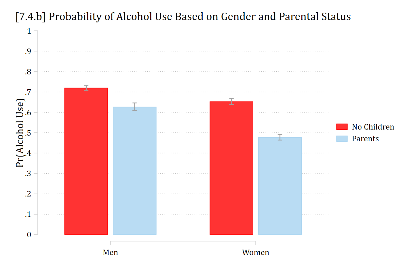
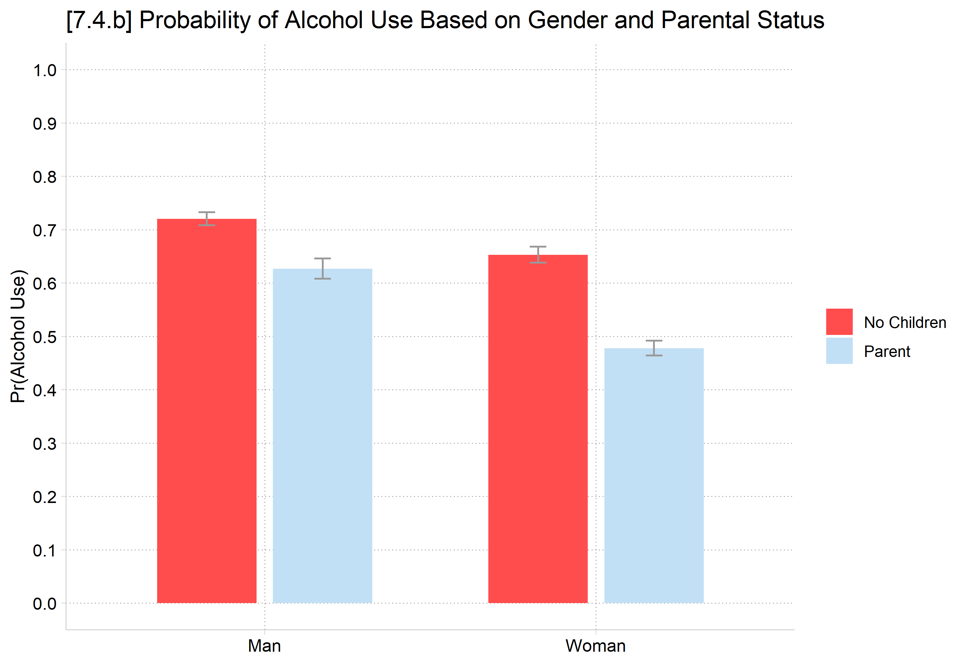
[7.4.b] Bar chart of the predicted probability of alcohol use for men and women, with and without children, with standard error bars. Men: about 0.72 without children and 0.63 as parents. Women: about 0.65 without children and 0.48 as parents. The parenthood gap is larger for women.

  • In R, use plot_predictions (default is dot plot)
plot_predictions(alc, by = c("woman", "parrole"),
  newdata = datagrid(woman = unique, parrole = unique, grid_type = "counterfactual"))
  • For a bar chart in R, save avg_predictions and pass to ggplot
# 7.4.b - Bar chart; parental status bars within gender, with SE bars (68% CIs)
pr <- avg_predictions(alc, by = c("woman", "parrole"), conf_level = .68,
  newdata = datagrid(woman = unique, parrole = unique, grid_type = "counterfactual"))

ggplot(pr, aes(x = woman, y = estimate, fill = parrole)) +
  geom_col(position = position_dodge(.7), width = .6) +
  geom_errorbar(aes(ymin = conf.low, ymax = conf.high), color = "gray60",
    position = position_dodge(.7), width = .1) +
  scale_y_continuous(breaks = seq(0, 1, .1), limits = c(0, 1)) +
  labs(title = "[7.4.b] Probability of Alcohol Use Based on Gender and Parental Status",
    x = NULL, y = "Pr(Alcohol Use)", fill = NULL)

[7.4.b] Bar chart of the predicted probability of alcohol use for men and women, with and without children, with standard error bars. Men: about 0.72 without children and 0.63 as parents. Women: about 0.65 without children and 0.48 as parents. The parenthood gap is larger for women.

Example bar chart to visualize interaction

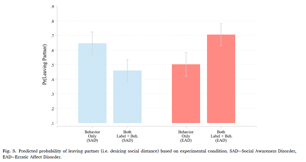
Figure 3 from Manago and Mize (2022): bar chart of the predicted probability of leaving a partner (desiring social distance) by experimental condition, for behavior only and for both a label and behavior, under Social Awareness Disorder and Erratic Affect Disorder, with confidence intervals.

*Figure from Manago and Mize 2022 SSR

Second differences (binary IVs)

*Predictions
est restore alcmod
(results alcmod are active now)
mtable, at(woman=(0 1) parrole=(0 1)) post
Expression: Pr(alcB), predict()

           |    woman   parrole     Pr(y)
 ----------+-----------------------------
         1 |        0         0     0.720
         2 |        0         1     0.627
         3 |        1         0     0.653
         4 |        1         1     0.478

Specified values where .n indicates no values specified with at()

           |  No at()
 ----------+---------
   Current |       .n
# Predictions
avg_predictions(alc, by = c("woman", "parrole"),
  newdata = datagrid(woman = unique, parrole = unique, grid_type = "counterfactual"))

 woman     parrole Estimate Std. Error    z Pr(>|z|)     S 2.5 % 97.5 %
 Man   No Children    0.720     0.0124 58.1   <0.001   Inf 0.696  0.745
 Man   Parent         0.627     0.0191 32.9   <0.001 785.7 0.590  0.664
 Woman No Children    0.653     0.0153 42.6   <0.001   Inf 0.623  0.683
 Woman Parent         0.478     0.0139 34.3   <0.001 855.5 0.450  0.505

Type: response

MEs and 2nd differences are based on these four values: each combination of the binary IVs

  • Identical procedure for calculating MEs and 2nd differences
    • Stata: mecompare and metest
    • R: avg_comparisons, then add hypothesis option
*MEs for effect of parenthood, by gender
mecompare parrole, by(woman) model(alcmod)
Predicting: Pr(alcB)
Marginal effects (N_alcmod=4307)

                                 |  ME #   Estimate         SE      P>|z|
---------------------------------+---------------------------------------
parrole                          |                                       
        Parent - No Children     |                                       
                             Man |     1     -0.093      0.023      0.000
                           Woman |     2     -0.175      0.021      0.000
*2nd difference: if parenthood has same effect for men and women
metest 2 - 1
                                 |  estimate         se     pvalue 
---------------------------------+--------------------------------
 parrole_woma~1 - parrole_woma~0 |    -0.082      0.030      0.007 
# MEs for effect of parenthood, by gender
avg_comparisons(alc, variables = "parrole", by = "woman",
  newdata = datagrid(woman = unique, grid_type = "counterfactual"))

 woman Estimate Std. Error     z Pr(>|z|)    S  2.5 % 97.5 %
 Man    -0.0935     0.0227 -4.12   <0.001 14.7 -0.138 -0.049
 Woman  -0.1753     0.0211 -8.32   <0.001 53.3 -0.217 -0.134

Term: parrole
Type: response
Comparison: Parent - No Children
# 2nd difference: if parenthood has same effect for men and women
avg_comparisons(alc, variables = "parrole", by = "woman",
  newdata = datagrid(woman = unique, grid_type = "counterfactual"),
  hypothesis = "b2 - b1 = 0")

 Hypothesis Estimate Std. Error    z Pr(>|z|)   S  2.5 %  97.5 %
    b2-b1=0  -0.0818     0.0303 -2.7  0.00698 7.2 -0.141 -0.0224

Type: response

Both men and women are less likely to drink alcohol if they are parents (both MEs p < 0.001). However, parenthood has a stronger negative effect on the probability of alcohol use for women (∆women = -0.175) than it does for men (∆men = -0.093; second difference = 0.082, p < 0.01).

Nominal X nominal interactions—example table

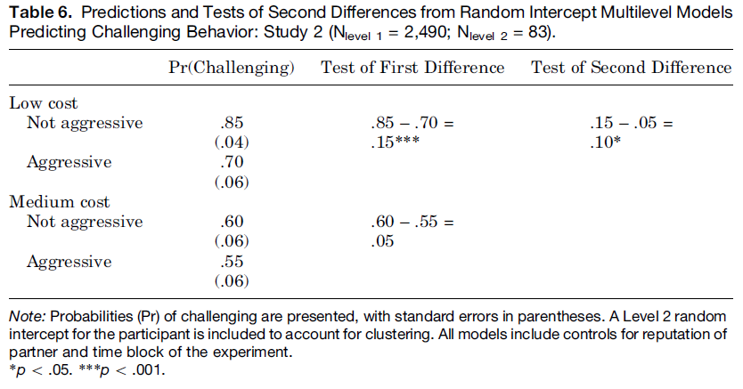
Table 6 from Benard, Berg, and Mize (2017): predictions and tests of second differences from random intercept multilevel models predicting challenging behavior. Low cost: not aggressive .85, aggressive .70, first difference .15 (p < .001); medium cost: not aggressive .60, aggressive .55, first difference .05; second difference .10 (p < .05).

Table from Benard, Berg, and Mize 2017 SPQ

Nominal X nominal interactions (multi-category IVs)

  • Testing for interaction is no more difficult when your nominal IV has more than two categories. However, the number of contrasts to present and test increase rapidly
///////////////////////////////////
// 3+ multi-category nominal IVs //
fre educ
educ -- Education Categories
-----------------------------------------------------------------------------
                                |      Freq.    Percent      Valid       Cum.
--------------------------------+--------------------------------------------
Valid   0 No High School Degree |        245       5.69       5.69       5.69
        1 High School Degree    |        780      18.11      18.11      23.80
        2 Some College          |       1766      41.00      41.00      64.80
        3 College Degree        |       1095      25.42      25.42      90.23
        4 Graduate Degree       |        421       9.77       9.77     100.00
        Total                   |       4307     100.00     100.00           
-----------------------------------------------------------------------------
qui logit alcB i.educ##i.woman c.age i.race c.income, or
estimates store alcedmod
# 3+ multi-category nominal IVs
frq(ah4, educ)
Education Categories (educ) <categorical> 
# total N=4307 valid N=4307 mean=3.15 sd=1.01

Value                 |    N | Raw % | Valid % | Cum. %
-------------------------------------------------------
No High School Degree |  245 |  5.69 |    5.69 |   5.69
High School Degree    |  780 | 18.11 |   18.11 |  23.80
Some College          | 1766 | 41.00 |   41.00 |  64.80
College Degree        | 1095 | 25.42 |   25.42 |  90.23
Graduate Degree       |  421 |  9.77 |    9.77 | 100.00
<NA>                  |    0 |  0.00 |    <NA> |   <NA>
alc2 <- glm(alcB ~ educ * woman + age + race + income, data = ah4,
  family = binomial(link = "logit"))
  • It is always a good idea to make a plot even if you do not present it in the paper
    • You can use bar charts here too—though they can become busy with lots of categories
    • Dot plots are best solution if graph would be too crowded with bars
*7.4.d - a dot plot with coefplot
est restore alcedmod
(results alcedmod are active now)
qui margins educ, at(woman=0) post
est store menprs
est restore alcedmod
(results alcedmod are active now)
qui margins educ, at(woman=1) post
est store womprs
*NOTE: Quirk is CIs are actually the 1st and 3rd thing being plotted;
*   for legend, label the 2nd and 4th (the markers)
coefplot menprs womprs, ///
    xtitle("Pr(Alcohol Use)") xlab(0(0.2)1) ///
    title("[7.4.d] Probability of Alcohol Use", size(medium)) ///
    subtitle("Interaction Effect: Gender X Educational Degree") ///
    legend(order(2 "Men" 4 "Women"))

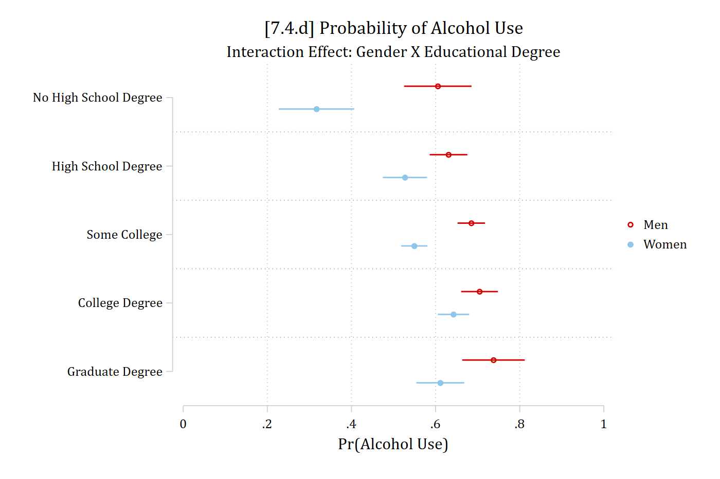
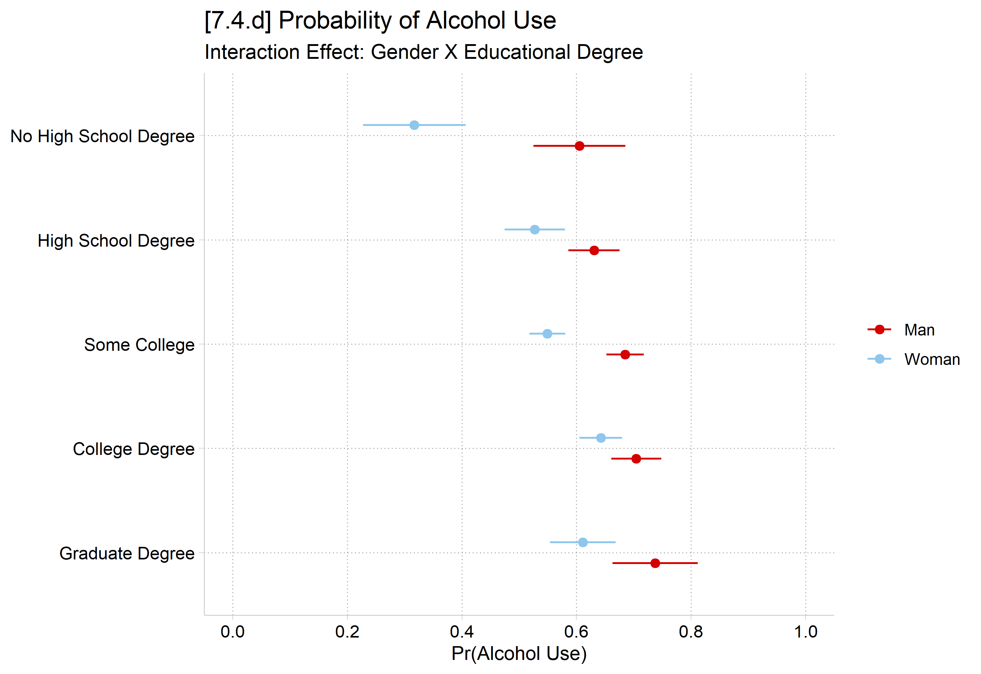
[7.4.d] Dot plot of the predicted probability of alcohol use with confidence intervals for men and women at each education level. Men's probabilities rise from about 0.60 (no high school degree) to about 0.74 (graduate degree). Women's are lower at every level: about 0.32 without a high school degree, then about 0.53 to 0.64 for the other degrees. The gender gap is largest without a high school degree.

# 7.4.d - a dot plot
pr2 <- avg_predictions(alc2, by = c("educ", "woman"),
  newdata = datagrid(educ = unique, woman = unique, grid_type = "counterfactual"))

ggplot(pr2, aes(x = estimate, y = educ, color = woman)) +
  geom_pointrange(aes(xmin = conf.low, xmax = conf.high),
    position = position_dodge(.4)) +
  scale_y_discrete(limits = rev) +
  scale_x_continuous(breaks = seq(0, 1, .2), limits = c(0, 1)) +
  labs(title = "[7.4.d] Probability of Alcohol Use",
    subtitle = "Interaction Effect: Gender X Educational Degree",
    x = "Pr(Alcohol Use)", y = NULL, color = NULL)

[7.4.d] Dot plot of the predicted probability of alcohol use with confidence intervals for men and women at each education level. Men's probabilities rise from about 0.60 (no high school degree) to about 0.74 (graduate degree). Women's are lower at every level: about 0.32 without a high school degree, then about 0.53 to 0.64 for the other degrees. The gender gap is largest without a high school degree.

*7.4.e - Bar chart with SE bars
est restore alcedmod
(results alcedmod are active now)
qui margins, at(educ=(0(1)4) woman=(0)) post
est store prmen
est restore alcedmod
(results alcedmod are active now)
qui margins, at(educ=(0(1)4) woman=(1)) post
est store prwom
coefplot prmen prwom, ///
    recast(bar) vertical barw(0.3) ciopts(recast(rcap) color(gs10)) ///
    citop level(68) ylab(0(.1)1) legend(order(1 "Men" 3 "Women")) ///
    xlab(1 `" "No HS" "Degree" "' 2 `" "High" "School" "' ///
        3 `" "Some" "College" "' 4 `" "College" "Degree" "' 5 `" "Graduate" "D
egree" "') ///
    ytitle("Pr(Alcohol Use)") scale(1.1) ///
    title("[7.4.e] Probability of Alcohol Use Based on Gender and Educational 
Attainment", span) ///
    subtitle("Interaction Effect: Gender X Educational Degree")

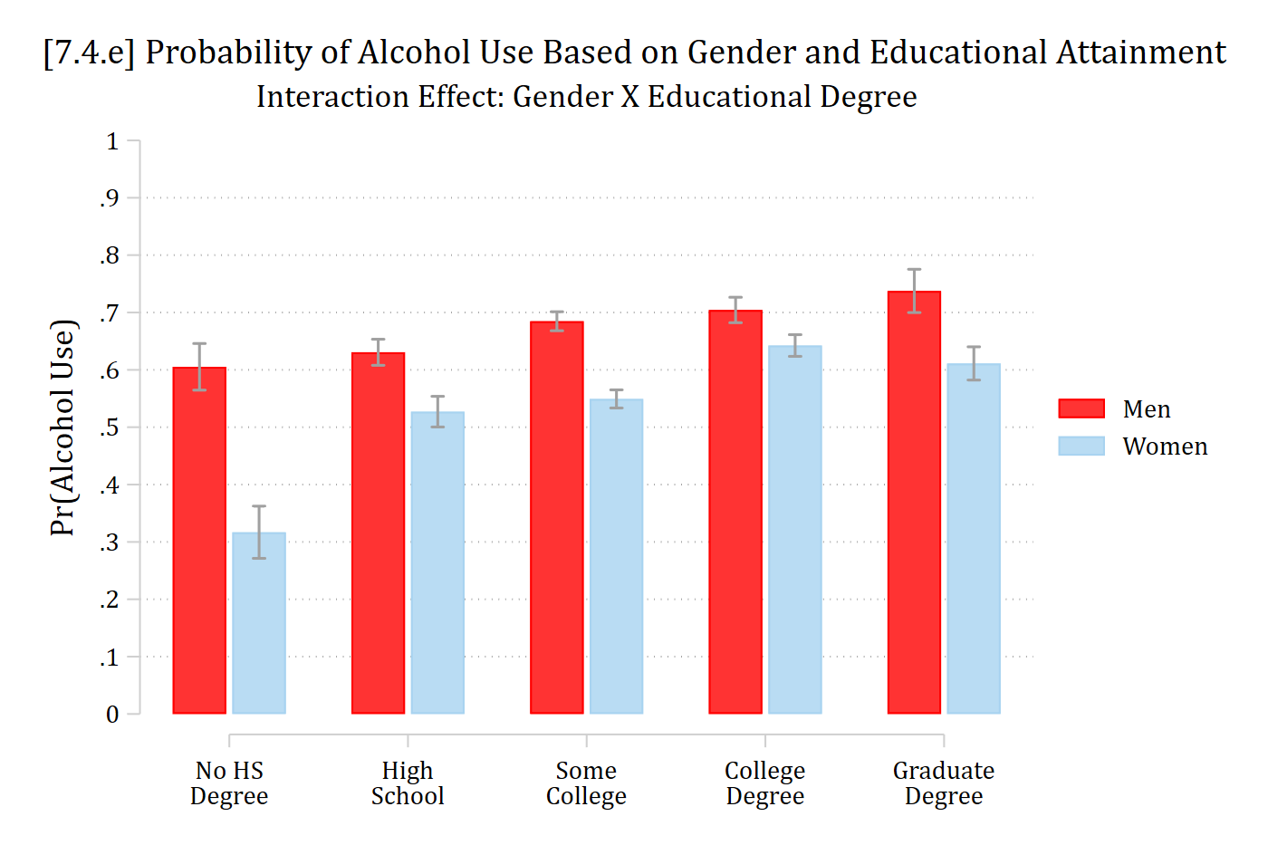
[7.4.e] Bar chart of the predicted probability of alcohol use for men and women at five education levels, with standard error bars. Men: about 0.60, 0.63, 0.68, 0.70, and 0.74 from no high school degree to graduate degree. Women: about 0.32, 0.53, 0.55, 0.64, and 0.61. Women are lower at every level, with the largest gap for those without a high school degree.

# 7.4.e - Bar chart with SE bars (68% CIs)
pr2 <- avg_predictions(alc2, by = c("educ", "woman"), conf_level = .68,
  newdata = datagrid(educ = unique, woman = unique, grid_type = "counterfactual"))

ggplot(pr2, aes(x = educ, y = estimate, fill = woman)) +
  geom_col(position = position_dodge(.7), width = .6) +
  geom_errorbar(aes(ymin = conf.low, ymax = conf.high), color = "gray60",
    position = position_dodge(.7), width = .1) +
  scale_x_discrete(labels = c("No HS\nDegree", "High\nSchool", "Some\nCollege",
    "College\nDegree", "Graduate\nDegree")) +
  scale_y_continuous(breaks = seq(0, 1, .1), limits = c(0, 1)) +
  labs(title = "[7.4.e] Probability of Alcohol Use Based on Gender and Educational Attainment",
    subtitle = "Interaction Effect: Gender X Educational Degree",
    x = NULL, y = "Pr(Alcohol Use)", fill = NULL)

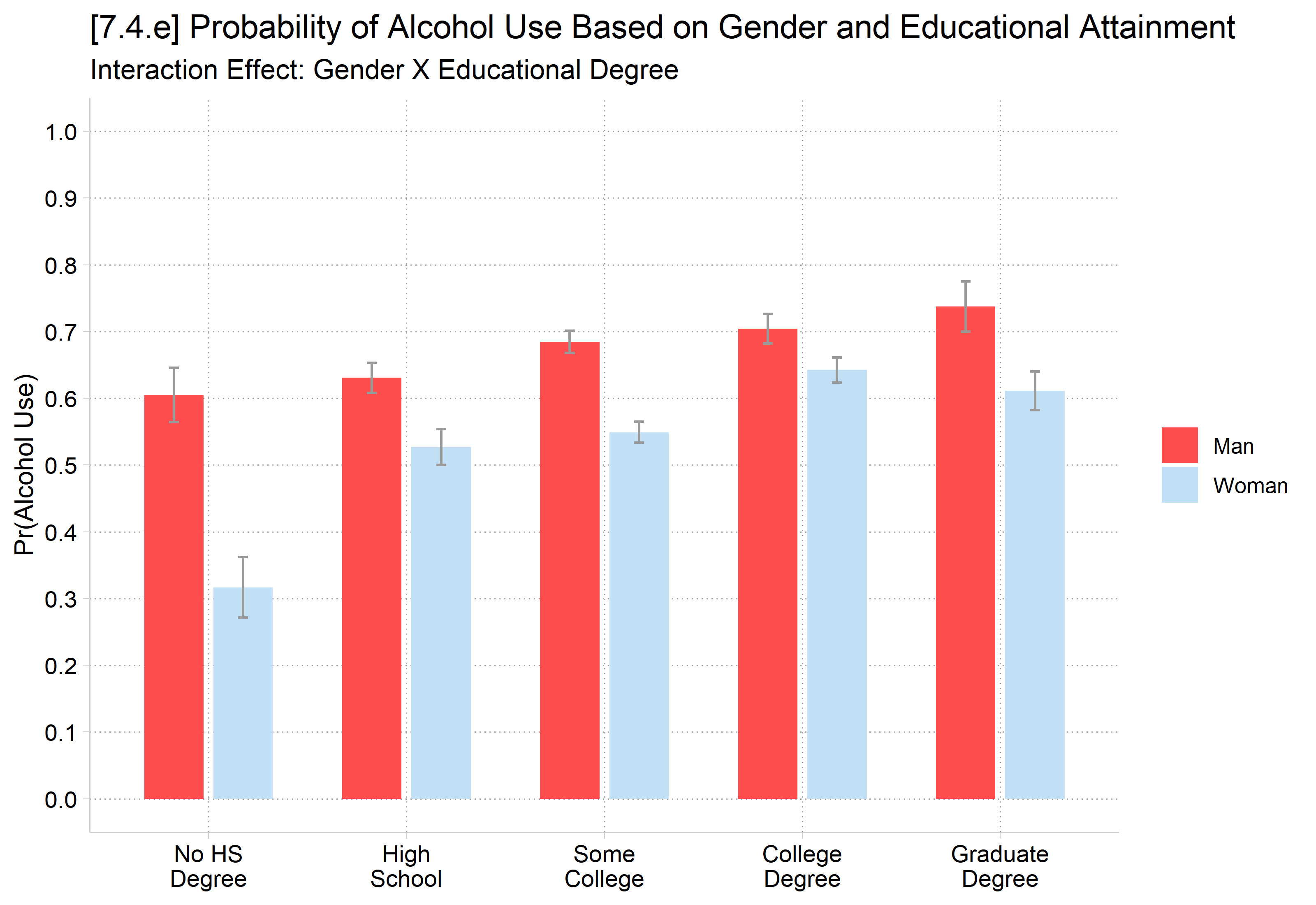
[7.4.e] Bar chart of the predicted probability of alcohol use for men and women at five education levels, with standard error bars. Men: about 0.60, 0.63, 0.68, 0.70, and 0.74 from no high school degree to graduate degree. Women: about 0.32, 0.53, 0.55, 0.64, and 0.61. Women are lower at every level, with the largest gap for those without a high school degree.

Joint tests of overall interaction effect

  • Because we have a binary (2 category) focal IV * a nominal (5 category) moderating IV, we have five 1st differences (MEs) to examine
  • To determine whether an interaction exists we need to examine the equality of the 1st differences
    • Often, useful to start with an omnibus or joint test before continuing to individual tests
      • I.e., Overall, are the 1st differences equivalent or different in size?
        • If different, proceed to examining what differences exist
      • But, sometimes a specific difference is hypothesized
        • If so, test this directly

Joint tests in Stata and R

  • In Stata, use mecompare and then metest for joint test (1 = 2 = 3 = … J)
// MEs (1st differences)
mecompare woman, by(educ) model(alcedmod)
Predicting: Pr(alcB)
Marginal effects (N_alcedmod=4307)

                                 |  ME #   Estimate         SE      P>|z|
---------------------------------+---------------------------------------
woman                            |                                       
                 Woman - Man     |                                       
           No High School Degree |     1     -0.288      0.061      0.000
              High School Degree |     2     -0.104      0.035      0.003
                    Some College |     3     -0.136      0.023      0.000
                  College Degree |     4     -0.062      0.029      0.033
                 Graduate Degree |     5     -0.126      0.048      0.008
*Start with a joint test of equality of all MEs
metest 1 = 2 = 3 = 4 = 5
Tests of equality

                                 |      chi2         df     pvalue 
---------------------------------+--------------------------------
                       1=2=3=4=5 |    12.390      4.000      0.015 
  • In R, use avg_comparisons for MEs
# MEs (1st differences)
avg_comparisons(alc2, variables = "woman", by = "educ",
  newdata = datagrid(educ = unique, grid_type = "counterfactual"))

                  educ Estimate Std. Error     z Pr(>|z|)    S  2.5 %   97.5 %
 No High School Degree   -0.288     0.0610 -4.73  < 0.001 18.7 -0.408 -0.16882
 High School Degree      -0.104     0.0353 -2.93  0.00335  8.2 -0.173 -0.03438
 Some College            -0.136     0.0232 -5.83  < 0.001 27.5 -0.181 -0.09000
 College Degree          -0.062     0.0290 -2.13  0.03286  4.9 -0.119 -0.00505
 Graduate Degree         -0.126     0.0475 -2.66  0.00781  7.0 -0.220 -0.03328

Term: woman
Type: response
Comparison: Woman - Man
  • For joint test, ask for 2nd diffs with hypothesis = ~reference and save as object
  • Then, test equality with hypotheses and option joint = TRUE
# Start with a joint test of equality of all MEs
diffs <- avg_comparisons(alc2, variables = "woman", by = "educ",
  newdata = datagrid(educ = unique, grid_type = "counterfactual"),
  hypothesis = ~ reference)
hypotheses(diffs, joint = TRUE, joint_test = "chisq")


Joint hypothesis test:
 b1 = 0
 b2 = 0
 b3 = 0
 b4 = 0
 
 ChiSq Pr(>|ChiSq|) Df
  12.4       0.0147  4

Type: response

Gender has a different effect across the levels of educational attainment, suggesting an interaction effect (joint test of MEs p = .015)

Hypothesized tests of 2nd differences

  • Whenever a specific 2nd difference is hypothesized, test that 2nd difference directly and don’t correct the p-value (Mize and Han 2025)

Ex H: Gender gaps in alcohol use will be larger for those who do not complete high school than for individuals with a high school degree

*If a specific 2nd diff is hypothesized, test that directly
metest 2 - 1
                                 |  estimate         se     pvalue 
---------------------------------+--------------------------------
     woman_educ_1 - woman_educ_0 |     0.185      0.070      0.008 
# If a specific 2nd diff is hypothesized, test that directly
avg_comparisons(alc2, variables = "woman", by = "educ",
  newdata = datagrid(educ = unique, grid_type = "counterfactual"),
  hypothesis = "b2 - b1 = 0")

 Hypothesis Estimate Std. Error    z Pr(>|z|)   S  2.5 % 97.5 %
    b2-b1=0    0.185     0.0702 2.63  0.00849 6.9 0.0472  0.322

Type: response

The gender gap, with women less likely to drink than men, is larger for those without a high school degree (MEwoman = -0.288) than for those with a high school degree (MEwoman = -0.104; 2nd diff. = 0.185, p < .01).

  • If you test for all 2nd differences, beware of Type I errors (false positives), and consider correcting the p-values for multiple comparisons (Mize and Han 2025)
    • Or, use an ME inequality to determine interaction (see below)

Nominal X nominal—example table

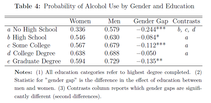
Table 4 from Mize (2019): probability of alcohol use by gender and education. Women: .336, .546, .567, .638, .594; men: .579, .630, .679, .688, .729 for no high school, high school, some college, college degree, and graduate degree. Gender gaps: -.244***, -.084*, -.112***, -.050, -.135**, with a column showing which gender gaps are significantly different.

*From Mize 2019

Nominal X nominal—example 2nd difference graph

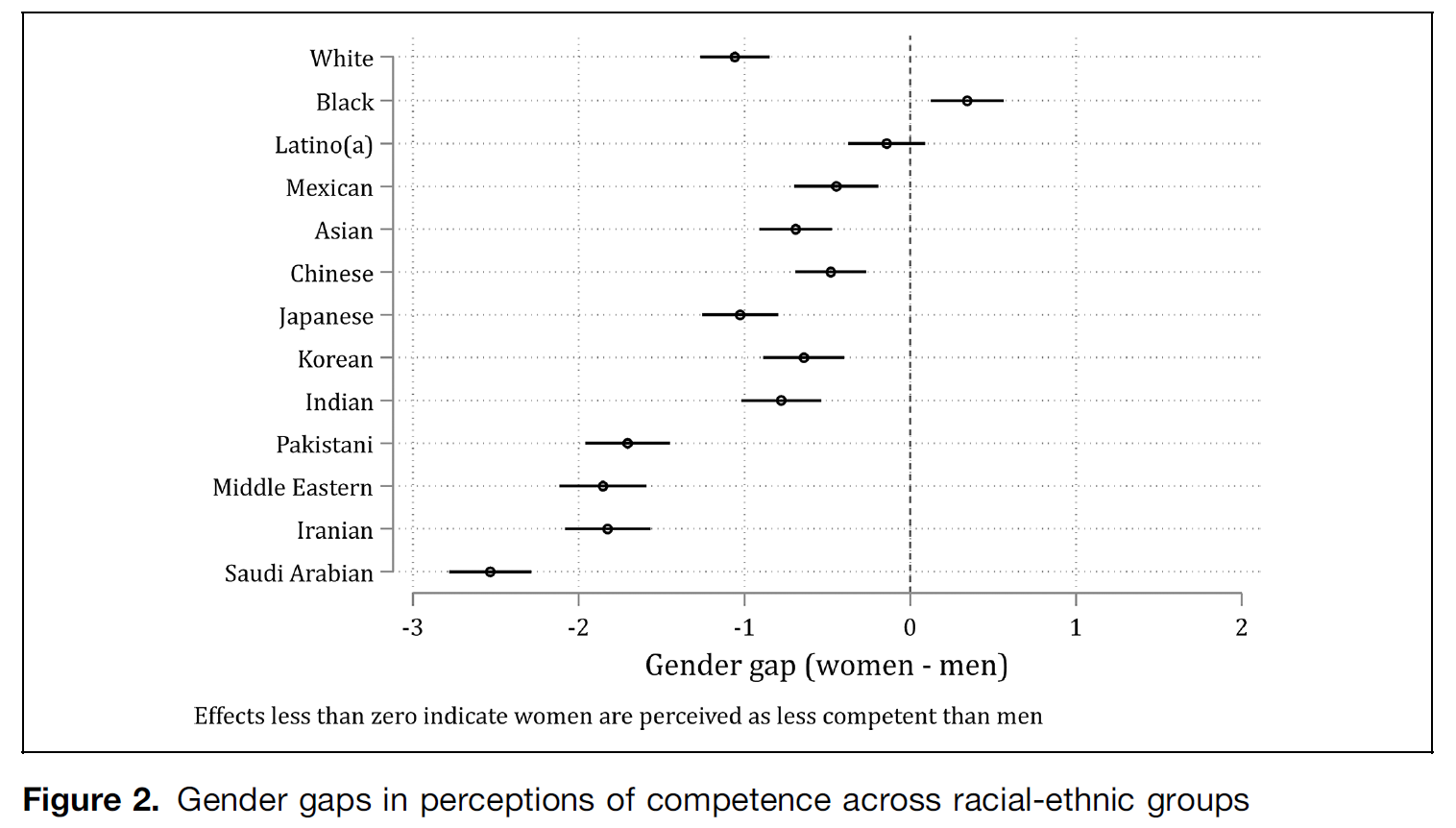
Figure 2 from Mize (2025): gender gaps (women minus men) in perceptions of competence across racial-ethnic groups, shown as points with confidence intervals for groups from White, Black, and Latino(a) to Middle Eastern, Iranian, and Saudi Arabian. Most gaps are negative, ranging from about -2.5 to 0.3.

*From Mize 2025

ME inequality tests of interaction

  • Sometimes, interest is in a nominal IV as a holistic construct
    • Consider these research questions

RQ: In the labor market, is there more racial-ethnic inequality among men or among women?

RQ: Has the role of religion in patterning social attitudes declined in recent years?

  • For these examples, race-ethnicity and religion as overall constructs are the focal IVs; not predicting specific category vs category comparisons
  • A benefit of using the ME inequality is it provides a single test and answer to the research question / hypothesis, so has no issue with multiple comparisons
  • The unweighted ME inequality* is simply the average of the (absolute values) of all pairwise comparisons (Mize and Han 2025)

\[unweighted\ ME\ inequality \equiv |unweighted\ average\ ME\ inequality|\]

\[= \frac{Sum\ of\ all\ |pairwise\ comparisons\ of\ MEs|}{\#\ of\ comparisons}\]

\[= \frac{\sum_{a = 1}^{L}\sum_{b = 2;\ b > a}^{L}\left| \eta\left( x_{k} = a,\ \mathbf{x}_{- k} = {\mathbf{x}_{- k}}^{*} \right) - \eta\left( x_{k} = b,\mathbf{x}_{- k} = {\mathbf{x}_{- k}}^{*} \right) \right|}{\frac{L(L - 1)}{2}}\]

  • Calculate the ME inequality at each value of the moderating IV
    • Test their equality as the 2nd difference test of interaction
  • In Stata, use the meinequality option on mecompare
    • Focal IV goes in varlist; moderating IV in by()
  • In R, use the meineq() function with avg_comparisons

*Mize and Han 2025 recommend the weighted version in most cases, but not this one, as weighting would conflate the changing religious compositions of the samples with the differences in MEs

ME inequality interaction example

  • DV: The variable spklgb asks respondents if they think an openly LGB person should be allowed to give a (pro-LGB?) speech in their community
    • The GSS spk* items measure support for various free speech rights
  • Moderating IV: year of survey
    • Binarized for simplicity: 1970s sample vs. recent sample (2012 or later)
  • Focal IV: Religious affiliation in 7 categories*
use "https://tdmize.github.io/data/data/cda_gss", clear
(cda_gss.dta |  GSS 1972-2021 CDA - Categorical Data Analysis | date created 202
> 3)
*DV: allow an LGB person to give a speech
gen spklgb = spkhomo
(28,919 missing values generated)
lab var spklgb "Allow LGB person to give speech"
lab def spklgb 0 "Don't Allow" 1 "Allow"
lab val spklgb spklgb
*Moderating IV: 1970s (1973-1980) vs recent (2012+) samples
gen recentyears = 0 if year <= 1980
(56,726 missing values generated)
replace recentyears = 1 if year >= 2012 & !missing(year)
(13,759 real changes made)
lab def recentyears 0 "1970s" 1 "2012+"
lab val recentyears recentyears
drop if missing(spklgb, recentyears, reltrad, age, woman)
(54,827 observations deleted)
fre spklgb recentyears reltrad
spklgb -- Allow LGB person to give speech
-------------------------------------------------------------------
                      |      Freq.    Percent      Valid       Cum.
----------------------+--------------------------------------------
Valid   0 Don't Allow |       3231      23.05      23.05      23.05
        1 Allow       |      10788      76.95      76.95     100.00
        Total         |      14019     100.00     100.00           
-------------------------------------------------------------------

recentyears
-------------------------------------------------------------
                |      Freq.    Percent      Valid       Cum.
----------------+--------------------------------------------
Valid   0 1970s |       6972      49.73      49.73      49.73
        1 2012+ |       7047      50.27      50.27     100.00
        Total   |      14019     100.00     100.00           
-------------------------------------------------------------

reltrad -- Religous Tradition
------------------------------------------------------------------------
                           |      Freq.    Percent      Valid       Cum.
---------------------------+--------------------------------------------
Valid   1 Evangelical      |       3323      23.70      23.70      23.70
        2 Mainline Prot    |       2918      20.81      20.81      44.52
        3 Black Protestant |       1088       7.76       7.76      52.28
        4 Catholic         |       3496      24.94      24.94      77.22
        5 Jewish           |        301       2.15       2.15      79.36
        6 Other Faith      |        693       4.94       4.94      84.31
        7 Nonaffiliated    |       2200      15.69      15.69     100.00
        Total              |      14019     100.00     100.00           
------------------------------------------------------------------------
gss <- read_dta("https://tdmize.github.io/data/data/cda_gss.dta")

# DV: allow an LGB person to give a speech
# Moderating IV: 1970s (1973-1980) vs recent (2012+) samples
lgb <- gss |>
  mutate(spklgb = spkhomo,
    recentyears = case_when(year <= 1980 ~ 0, year >= 2012 ~ 1)) |>
  select(spklgb, recentyears, reltrad, age, woman)
lgb <- lgb[complete.cases(lgb), ] |>
  mutate(recentyears = factor(recentyears, levels = 0:1, labels = c("1970s", "2012+")),
    across(c(reltrad, woman), as_factor))

frq(lgb, spklgb, recentyears, reltrad)
allow homosexual to speak (spklgb) <numeric> 
# total N=14019 valid N=14019 mean=0.77 sd=0.42

Value |       Label |     N | Raw % | Valid % | Cum. %
------------------------------------------------------
    0 | Don't Allow |  3231 | 23.05 |   23.05 |  23.05
    1 |       Allow | 10788 | 76.95 |   76.95 | 100.00
 <NA> |        <NA> |     0 |  0.00 |    <NA> |   <NA>

recentyears <categorical> 
# total N=14019 valid N=14019 mean=1.50 sd=0.50

Value |    N | Raw % | Valid % | Cum. %
---------------------------------------
1970s | 6972 | 49.73 |   49.73 |  49.73
2012+ | 7047 | 50.27 |   50.27 | 100.00
<NA>  |    0 |  0.00 |    <NA> |   <NA>

Religous Tradition (reltrad) <categorical> 
# total N=14019 valid N=14019 mean=3.39 sd=2.07

Value            |    N | Raw % | Valid % | Cum. %
--------------------------------------------------
Evangelical      | 3323 | 23.70 |   23.70 |  23.70
Mainline Prot    | 2918 | 20.81 |   20.81 |  44.52
Black Protestant | 1088 |  7.76 |    7.76 |  52.28
Catholic         | 3496 | 24.94 |   24.94 |  77.22
Jewish           |  301 |  2.15 |    2.15 |  79.36
Other Faith      |  693 |  4.94 |    4.94 |  84.31
Nonaffiliated    | 2200 | 15.69 |   15.69 | 100.00
<NA>             |    0 |  0.00 |    <NA> |   <NA>
qui logit spklgb i.reltrad##i.recentyears c.age i.woman
est store lgbmod
*7.4.f - Predictions by religious tradition in each period
qui margins, at(recentyears=(0 1))
matrix avgpr = r(b)
est restore lgbmod
(results lgbmod are active now)
qui margins reltrad, at(recentyears=0) post
est store pr1970s
est restore lgbmod
(results lgbmod are active now)
qui margins reltrad, at(recentyears=1) post
est store pr2012
coefplot pr1970s pr2012, xtitle("Pr(Support LGB free speech)") ///
    xline(`=avgpr[1,1]', lpat(dash) lcol(red)) ///
    xline(`=avgpr[1,2]', lpat(dash) lcol(eltblue)) ///
    legend(order(2 "1970s" 4 "2012+") title("Sample")) ///
    title("[7.4.f] Effect of religious affiliation on support for LGB speech, 
over time")

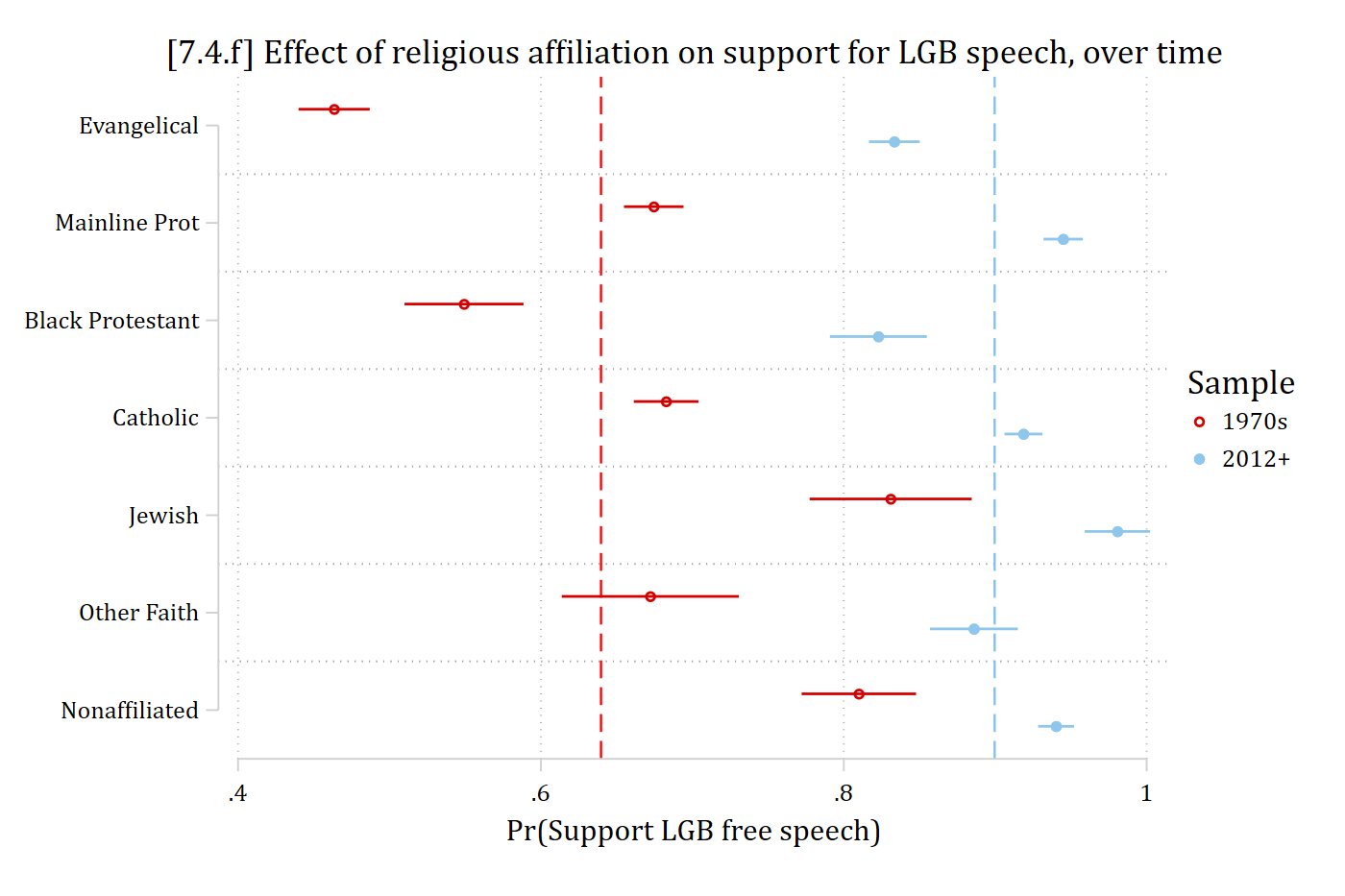
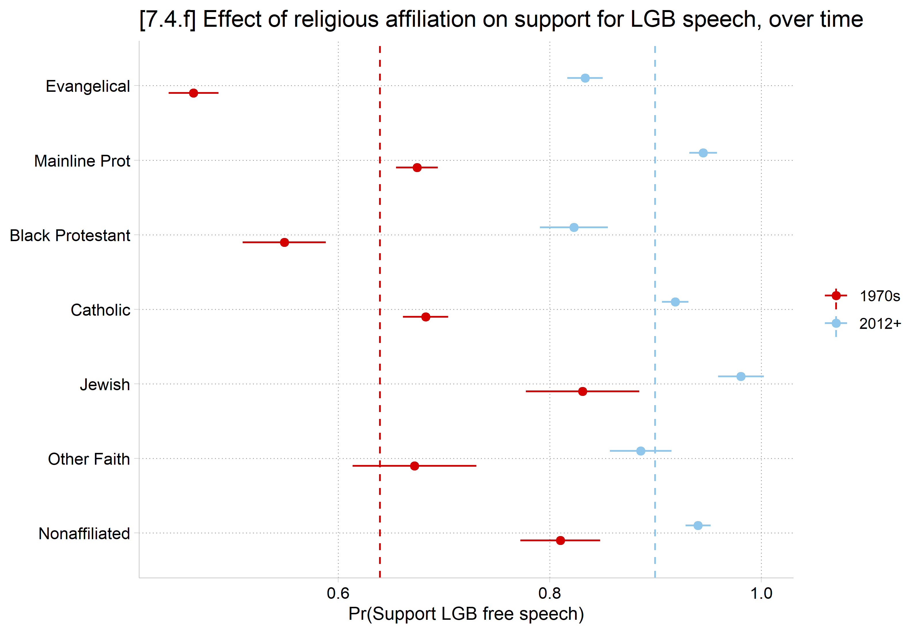
[7.4.f] Dot plot of the predicted probability of supporting an LGB person's free speech by religious tradition, in the 1970s and in 2012 or later, with dashed lines at each period's average. In the 1970s probabilities range from about 0.46 (Evangelical) and 0.55 (Black Protestant) to about 0.83 (Jewish), around an average near 0.64. In 2012 or later all traditions are higher, from about 0.82 to 0.98, around an average near 0.90, and the traditions are much closer together.

lgbmod <- glm(spklgb ~ reltrad * recentyears + age + woman, data = lgb,
  family = binomial(link = "logit"))

# 7.4.f - Predictions by religious tradition in each period
avgpr <- avg_predictions(lgbmod, by = "recentyears",
  newdata = datagrid(recentyears = unique, grid_type = "counterfactual"))
pr <- avg_predictions(lgbmod, by = c("reltrad", "recentyears"),
  newdata = datagrid(reltrad = unique, recentyears = unique, grid_type = "counterfactual"))

ggplot(pr, aes(x = estimate, y = reltrad, color = recentyears)) +
  geom_vline(data = avgpr, aes(xintercept = estimate, color = recentyears),
    linetype = "dashed") +
  geom_pointrange(aes(xmin = conf.low, xmax = conf.high),
    position = position_dodge(.4)) +
  scale_y_discrete(limits = rev) +
  labs(title = "[7.4.f] Effect of religious affiliation on support for LGB speech, over time",
    x = "Pr(Support LGB free speech)", y = NULL, color = "Sample")

[7.4.f] Dot plot of the predicted probability of supporting an LGB person's free speech by religious tradition, in the 1970s and in 2012 or later, with dashed lines at each period's average. In the 1970s probabilities range from about 0.46 (Evangelical) and 0.55 (Black Protestant) to about 0.83 (Jewish), around an average near 0.64. In 2012 or later all traditions are higher, from about 0.82 to 0.98, around an average near 0.90, and the traditions are much closer together.

*The distribution of religious affiliation has changed substantially over time, hence the decision to use the unweighted ME inequality here

mecompare reltrad, by(recentyears) meinequality(unweighted) model(lgbmod)
Predicting: Pr(spklgb)
Marginal effects (N_lgbmod=14019)

                                 |  ME #   Estimate         SE      P>|z|
---------------------------------+---------------------------------------
reltrad                          |                                       
              Unwgt ME Ineq.     |                                       
                           1970s |     1      0.156      0.010      0.000
                           2012+ |     2      0.072      0.006      0.000
    Mainline Pr - Evangelica     |                                       
                           1970s |     3      0.211      0.016      0.000
                           2012+ |     4      0.112      0.011      0.000
    Black Prote - Evangelica     |                                       
                           1970s |     5      0.086      0.023      0.000
                           2012+ |     6     -0.011      0.018      0.567
      Catholic - Evangelical     |                                       
                           1970s |     7      0.219      0.016      0.000
                           2012+ |     8      0.085      0.011      0.000
        Jewish - Evangelical     |                                       
                           1970s |     9      0.368      0.030      0.000
                           2012+ |    10      0.147      0.014      0.000
    Other Faith - Evangelica     |                                       
                           1970s |    11      0.209      0.032      0.000
                           2012+ |    12      0.053      0.017      0.002
    Nonaffiliat - Evangelica     |                                       
                           1970s |    13      0.347      0.023      0.000
                           2012+ |    14      0.107      0.011      0.000
# ME inequality functions
source("https://raw.githubusercontent.com/tdmize/Rfunctions/main/ME_helper_functions.R")

meq <- avg_comparisons(lgbmod, variables = list(reltrad = "pairwise"), by = "recentyears",
  newdata = datagrid(recentyears = unique, grid_type = "counterfactual"),
  hypothesis = meineq(lgbmod, weighted = FALSE))
meq

 recentyears Estimate Std. Error    z Pr(>|z|)     S  2.5 % 97.5 %
       1970s   0.1557    0.01047 14.9   <0.001 163.8 0.1351 0.1762
       2012+   0.0715    0.00618 11.6   <0.001 100.4 0.0594 0.0836

Term: reltrad
Type: response

Individuals from different religious traditions differed by about 16 percentage points in their opinions in the 1970s.

In more recent years, religious traditions differ by only about 7 percentage points, on average.

metest 2 - 1
                                 |  estimate         se     pvalue 
---------------------------------+--------------------------------
 reltrad_MEin~1 - reltrad_MEin~0 |    -0.084      0.012      0.000 
hypotheses(meq, hypothesis = "b2 - b1 = 0")

 Hypothesis Estimate Std. Error     z Pr(>|z|)    S  2.5 %  97.5 %
    b2-b1=0  -0.0841     0.0122 -6.92   <0.001 37.7 -0.108 -0.0603

Religious tradition had a larger effect on patterning opinions in the 1970s than it does in more recent years; the overall effect has declined by over 8 percentage points (2nd differences in ME inequalities, p < .001).
Back to top