3.5 Interpreting Predictions

\[Logit: \Pr(y_{i} = 1\,|\,\mathbf{x}_{i}) = \Lambda(\mathbf{x}_{i}\widehat{\boldsymbol{\beta}}) = \frac{\exp(\mathbf{x}_{i}\widehat{\boldsymbol{\beta}})}{1 + \exp(\mathbf{x}_{i}\widehat{\boldsymbol{\beta}})}\]

\[Probit: \Pr(y_{i} = 1\,|\,\mathbf{x}_{i}) = \Phi(\mathbf{x}_{i}\widehat{\boldsymbol{\beta}}) = \int_{-\infty}^{\mathbf{x}_{i}\widehat{\boldsymbol{\beta}}} \frac{1}{\sqrt{2\pi}}\exp\left(-\frac{t^{2}}{2}\right)dt\]

Possible range of predicted probabilities

  • The logit and probit functional form constrain predicted probabilities to be between 0 and 1
    • No non-sensical prediction problems like in the LPM
    • Consider the ANES 2020 voting intentions data
use "https://tdmize.github.io/data/data/cda_anes", clear
(American National Election Study 2020 - Pre-election | CDA | 2021-09-26)
drop if missing(age, hhincome, woman, lgb, race4, ///
    edyrs, relimport, wrongtrack)
(948 observations deleted)
qui regress vote_trump age hhincome i.woman i.lgb i.race4 ///
    edyrs i.relimport i.wrongtrack
* Make prediction for highly educated black woman
mtable, at(woman=1 race4=2 edyrs=20 relimport=5 wrongtrack=1)
Expression: Linear prediction, predict()

      xb
--------
  -0.301

Specified values of covariates

           |    woman     race4     edyrs  relimport  wrongtrack
 ----------+----------------------------------------------------
   Current |        1         2        20          5           1
qui logit vote_trump age hhincome i.woman i.lgb i.race4 ///
    edyrs i.relimport i.wrongtrack
* Make prediction for highly educated black woman
mtable, at(woman=1 race4=2 edyrs=20 relimport=5 wrongtrack=1)
Expression: Pr(vote_trump), predict()

   Pr(y)
--------
   0.004

Specified values of covariates

           |    woman     race4     edyrs  relimport  wrongtrack
 ----------+----------------------------------------------------
   Current |        1         2        20          5           1
library(haven)           # import Stata data and labels
library(dplyr)           # data manipulation
library(sjmisc)          # frequency tables
library(ggplot2)         # graphs
library(marginaleffects) # predictions and marginal effects
library(questionr)       # odds ratios
library(cleanplots)      # graph scheme
cleanplots_defaults()

# Center changes in continuous IVs on each observation's value
options(marginaleffects_contrast_direction = "center")

anes <- read_dta("https://tdmize.github.io/data/data/cda_anes.dta")

# Drop any missing data on the model IVs
anes <- anes[complete.cases(anes[c("age", "hhincome", "woman", "lgb", "race4",
  "edyrs", "relimport", "wrongtrack")]), ]

# Treat binary/nominal variables as factors using their value labels
anes <- anes |>
  mutate(woman = as_factor(woman), lgb = as_factor(lgb), race4 = as_factor(race4),
    relimport = as_factor(relimport), wrongtrack = as_factor(wrongtrack),
    college = as_factor(college)) |>
  droplevels()

lpm1 <- lm(vote_trump ~ age + hhincome + woman + lgb + race4 + edyrs + relimport +
  wrongtrack, data = anes)

# Make prediction for highly educated black woman
avg_predictions(lpm1, newdata = datagrid(woman = "Woman", race4 = "Black", edyrs = 20,
  relimport = "5. Not important at all", wrongtrack = "Wrong track",
  grid_type = "counterfactual"))

 Estimate Std. Error   z Pr(>|z|)     S  2.5 % 97.5 %
   -0.301     0.0216 -14   <0.001 145.1 -0.344 -0.259

Type: response
logit1 <- glm(vote_trump ~ age + hhincome + woman + lgb + race4 + edyrs + relimport +
  wrongtrack, family = binomial(link = "logit"), data = anes)

# Make prediction for highly educated black woman
avg_predictions(logit1, newdata = datagrid(woman = "Woman", race4 = "Black", edyrs = 20,
  relimport = "5. Not important at all", wrongtrack = "Wrong track",
  grid_type = "counterfactual"))

 Estimate Std. Error    z Pr(>|z|)    S   2.5 %  97.5 %
  0.00355   0.000803 4.42   <0.001 16.6 0.00197 0.00512

Type: response

The LPM produces a non-sensical -.30 predicted probability that a highly educated black woman would vote for Trump

A logit model produces a reasonable 0.004 pr. prob – indicating the woman is highly unlikely to vote for Trump

qui regress vote_trump age hhincome i.woman i.lgb i.race4 ///
    edyrs i.relimport i.wrongtrack feel_trump
qui margins, at(feel_trump=(0(5)100)) saving(lpm_tr, replace)
qui logit vote_trump age hhincome i.woman i.lgb i.race4 ///
    edyrs i.relimport i.wrongtrack feel_trump
qui margins, at(feel_trump=(0(5)100)) saving(logit_tr, replace)
sort feel_trump // needed for ensuing plot
lowess vote_trump feel_trump, bwidth(0.15) gen(low_trump) nograph
combomarginsplot lpm_tr logit_tr, ///
    yline(0 1) recastci(rline) ciopt(lpat(dash) color(*.5)) ///
    plotopt(msym(none) lwid(medthick)) ///
    addplot(connected low_trump feel_trump, ylab(0(0.2)1) xlab(0(10)100) ///
    msym(none) lcol(gs8) lwid(medthick) legend(order(3 "LPM" 4 "Logit" 5 "Lowe
ss")) ///
    title("[3.11.b2] Predicted probability of voting for Trump based on feelin
gs toward Trump", size(medium)) ///
    subtitle("Comparison of linear probability model (LPM), logit, and lowess"
, size(small)) ///
    ytitle("Pr(voting for Trump)"))
  Variables that uniquely identify margins: feel_trump _filenumber

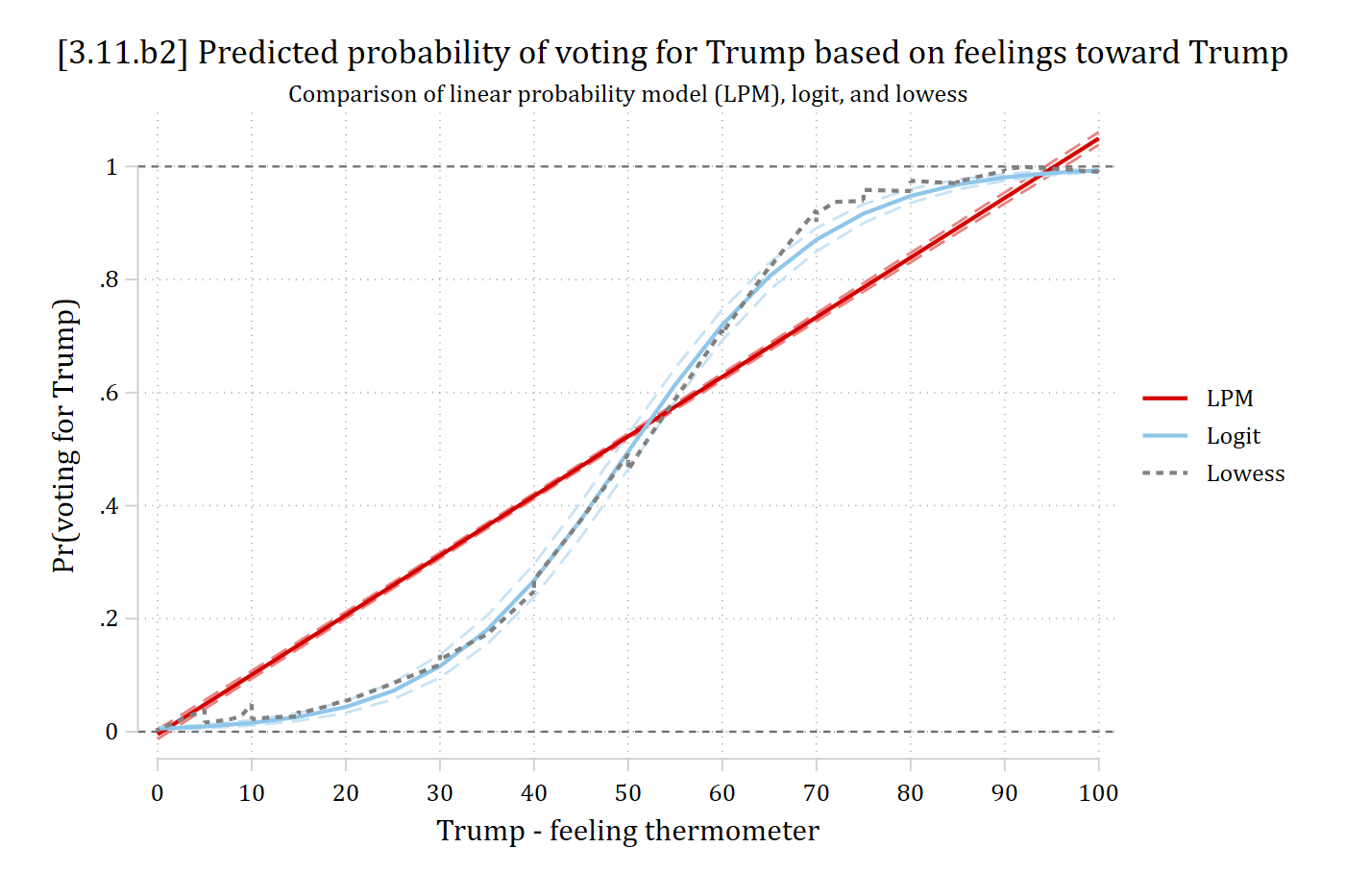
Predicted probability of voting for Trump by the Trump feeling thermometer from the LPM, the logit, and the lowess: the logit's S-curve follows the lowess closely while the straight LPM line does not.

lpm2 <- lm(vote_trump ~ age + hhincome + woman + lgb + race4 + edyrs + relimport +
  wrongtrack + feel_trump, data = anes)
lpm_tr <- avg_predictions(lpm2, by = "feel_trump",
  newdata = datagrid(feel_trump = seq(0, 100, 5), grid_type = "counterfactual"))

logit2 <- glm(vote_trump ~ age + hhincome + woman + lgb + race4 + edyrs + relimport +
  wrongtrack + feel_trump, family = binomial(link = "logit"), data = anes)
logit_tr <- avg_predictions(logit2, by = "feel_trump",
  newdata = datagrid(feel_trump = seq(0, 100, 5), grid_type = "counterfactual"))

trump_prs <- bind_rows(LPM = lpm_tr, Logit = logit_tr, .id = "model")

ggplot(trump_prs, aes(x = feel_trump, y = estimate, color = model)) +
  geom_line(linewidth = 1) +
  geom_line(aes(y = conf.low), linetype = "dashed") +
  geom_line(aes(y = conf.high), linetype = "dashed") +
  geom_smooth(data = anes, aes(x = feel_trump, y = vote_trump, color = "Smoothed"),
    se = FALSE) +
  geom_hline(yintercept = c(0, 1), linetype = "dashed") +
  scale_color_discrete(limits = c("LPM", "Logit", "Smoothed")) +
  scale_x_continuous(breaks = seq(0, 100, 10)) +
  labs(title = "[3.11.b2] Predicted probability of voting for Trump based on feelings toward Trump",
    subtitle = "Comparison of linear probability model (LPM), logit, and smoothed proportions",
    x = "Trump - feeling thermometer", y = "Pr(voting for Trump)", color = NULL)

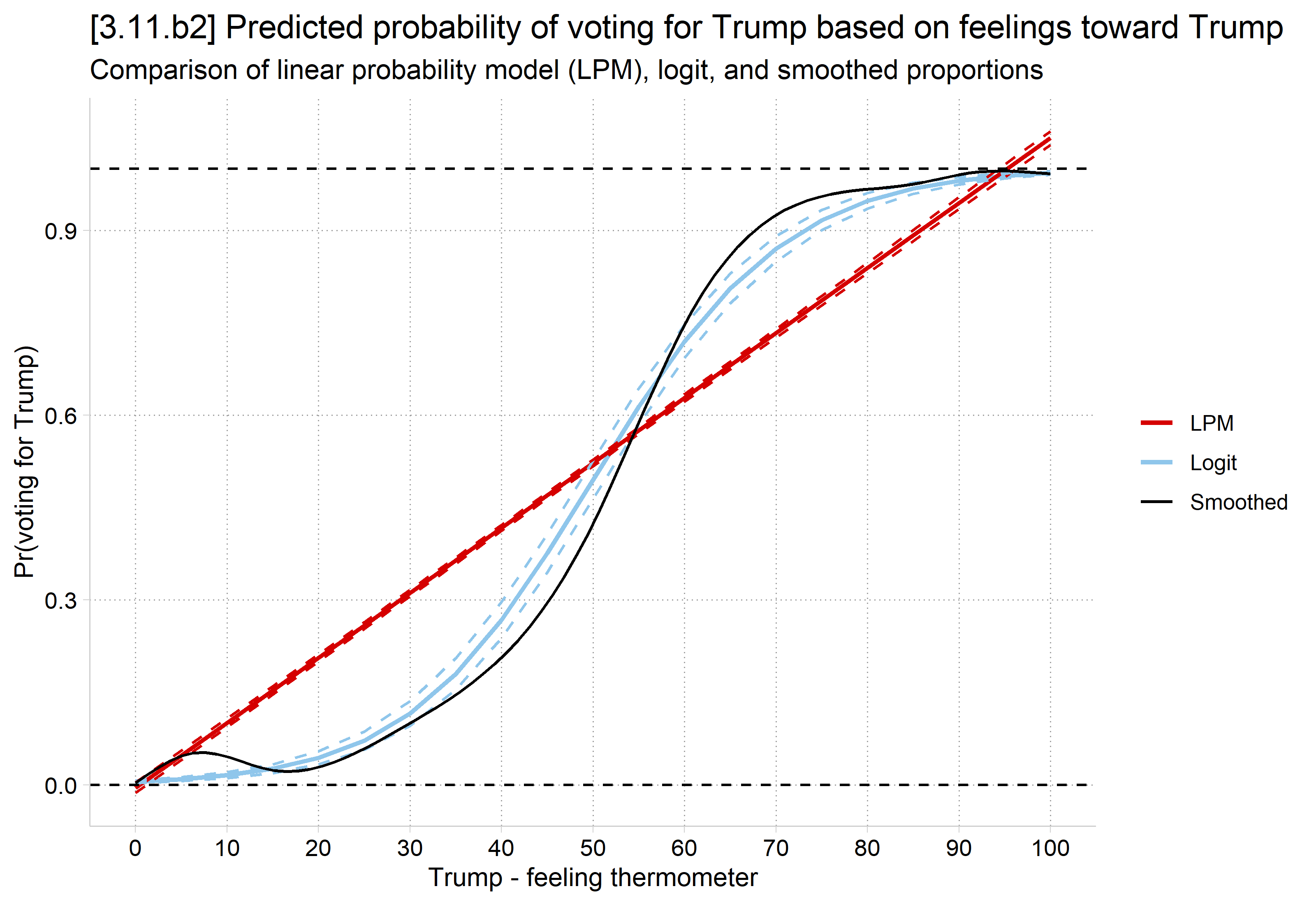
Predicted probability of voting for Trump by the Trump feeling thermometer from the LPM, the logit, and smoothed proportions: the logit's S-curve follows the smoothed curve closely while the straight LPM line does not.

On the support of the data: logit vs LPM

Where is your data? Where do you want to examine the effects?

* Add distribution of feel_trump (IV) to plot
qui logit vote_trump age hhincome i.woman i.lgb i.race4 ///
    edyrs i.relimport i.wrongtrack feel_trump
qui margins, at(feel_trump=(0(5)100))
marginsplot, ///
    xlab(0(10)100) ///
    ytitle("Pr(Voting for Trump)") ///
    recastci(rline) ciopt(lpat(dash) color(*.5)) ///
    plotopt(msym(none) lwid(medthick)) ///
    title("[3.5.b] Predicted probability of voting for Trump based on feelings
 toward Trump") ///
    subtitle("Kernel density plot show distribution of feeling thermometer", s
ize(small)) ///
    addplot(kdensity feel_trump, ///
    ylab(-.3 " " 0(.2)1) yaxis(2) yscale(range(0 0.1) off alt axis(2))) ///
    legend(off)
Variables that uniquely identify margins: feel_trump

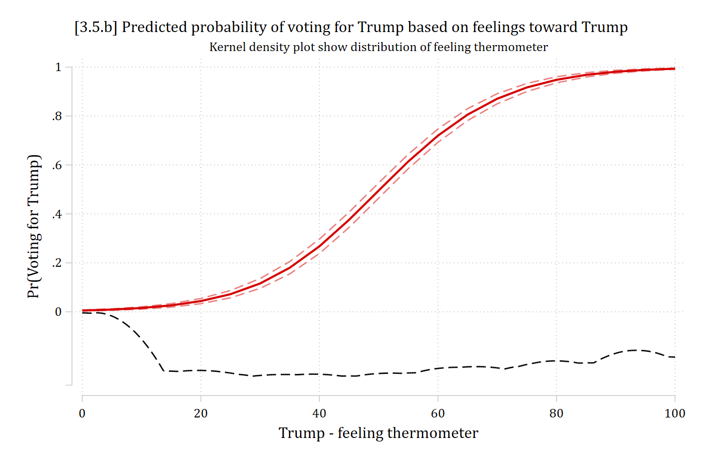
Logit predicted probability of voting for Trump by the Trump feeling thermometer, an S-curve, with a kernel density of the thermometer beneath it: most observations are at the low and high ends of the thermometer, where the curve is flat.

ggplot(logit_tr, aes(x = feel_trump, y = estimate)) +
  geom_line(linewidth = 1) +
  geom_line(aes(y = conf.low), linetype = "dashed", color = "gray60") +
  geom_line(aes(y = conf.high), linetype = "dashed", color = "gray60") +
  # kernel density of feel_trump, scaled to sit below the predictions
  geom_density(data = anes, aes(x = feel_trump, y = after_stat(-0.3 + 0.25 * density / max(density))),
    inherit.aes = FALSE, color = "gray40") +
  scale_x_continuous(breaks = seq(0, 100, 10)) +
  scale_y_continuous(breaks = seq(0, 1, 0.2)) +
  labs(title = "[3.5.b] Predicted probability of voting for Trump based on feelings toward Trump",
    subtitle = "Kernel density plot show distribution of feeling thermometer",
    x = "Trump - feeling thermometer", y = "Pr(Voting for Trump)")

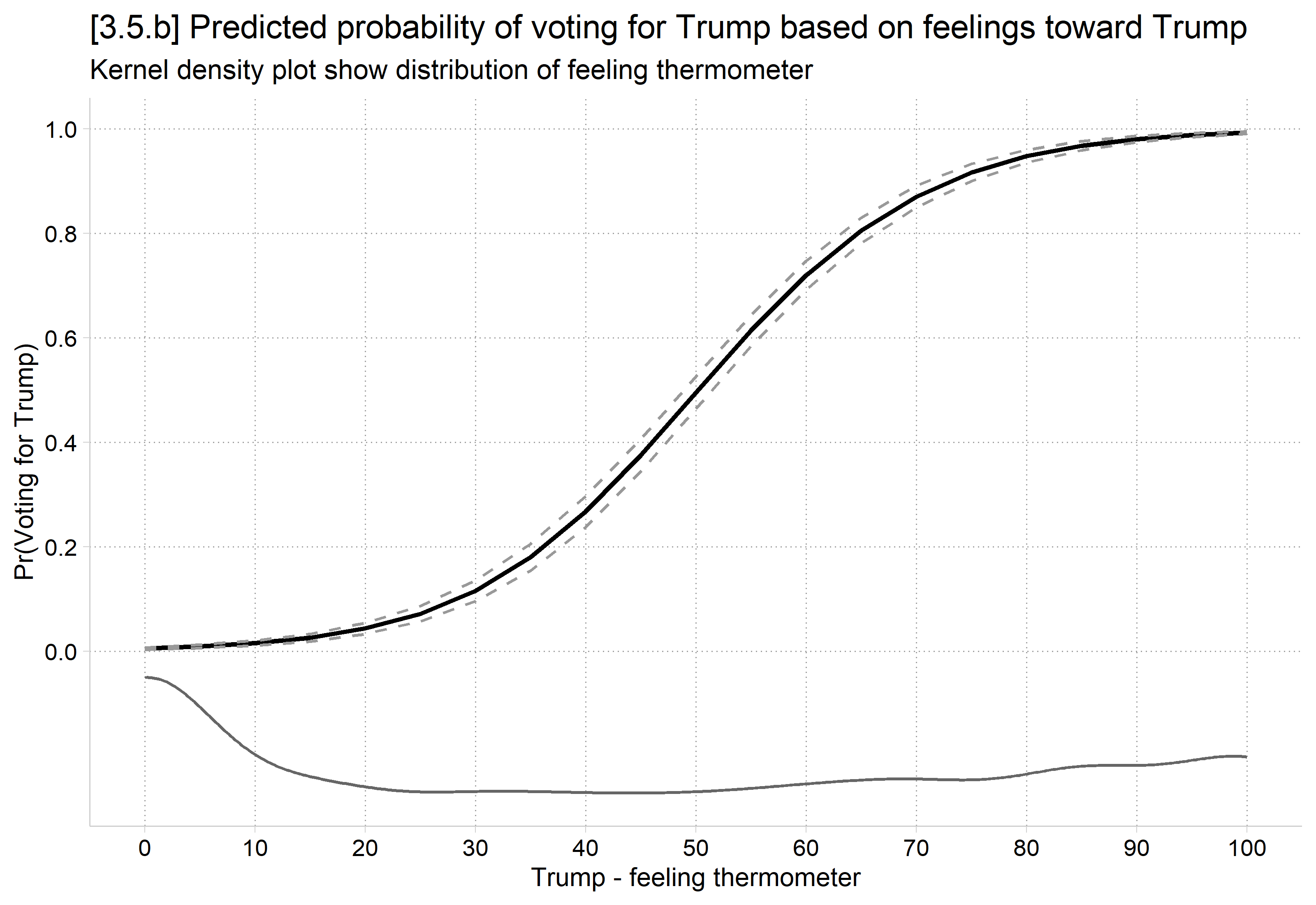
Logit predicted probability of voting for Trump by the Trump feeling thermometer, an S-curve, with a kernel density of the thermometer beneath it: most observations are at the low and high ends of the thermometer, where the curve is flat.

  • We can compare +SD effects across the LPM and logit
// Compare LPM to logit
qui regress vote_trump c.feel_trump age hhincome i.woman i.lgb i.race4 ///
    i.college i.relimport i.wrongtrack
est store lpm
qui logit vote_trump c.feel_trump age hhincome i.woman i.lgb i.race4 ///
    i.college i.relimport i.wrongtrack
est store logit_m
* Compare average effects across models
mecompare feel_trump, models(lpm logit_m) amount(sd)
mecompare uses vce(robust) for all models. Standard errors from mecompare will d
> iffer from the specified model(s) because vce(robust) was not used on at least
>  one of the models specified in the models( ) option. We strongly recommend re
> fitting the first (regress) and second (logit) models with vce(robust). See vc
> e_option for details on vce(robust).

Predicting: Linear prediction (lpm), Pr(vote_trump) (logit_m)
Marginal effects and cross-model differences (N_lpm=6695) (N_logit_m=6695)

                                 |  ME #   Estimate  Robust SE      P>|z|
---------------------------------+---------------------------------------
feel trump + SD (centered)       |                                       
                             lpm |     1      0.432      0.004      0.000
                         logit m |     2      0.166      0.004      0.000
                      Difference |     3      0.266      0.004      0.000
# Compare LPM to logit (keep the observations used in both models)
anes_m <- anes[complete.cases(anes[c("vote_trump", "feel_trump", "college")]), ]

lpm <- lm(vote_trump ~ feel_trump + age + hhincome + woman + lgb + race4 + college +
  relimport + wrongtrack, data = anes_m)

logit_m <- glm(vote_trump ~ feel_trump + age + hhincome + woman + lgb + race4 + college +
  relimport + wrongtrack, family = binomial(link = "logit"), data = anes_m)

# Compare average effects across models
sd_feel <- sd(anes_m$feel_trump)
avg_comparisons(lpm, variables = list(feel_trump = sd_feel))

 Estimate Std. Error   z Pr(>|z|)   S 2.5 % 97.5 %
    0.432    0.00353 123   <0.001 Inf 0.425  0.439

Term: feel_trump
Type: response
Comparison: +40.9766662288769
avg_comparisons(logit_m, variables = list(feel_trump = sd_feel))

 Estimate Std. Error    z Pr(>|z|)   S 2.5 % 97.5 %
    0.166    0.00341 48.6   <0.001 Inf 0.159  0.172

Term: feel_trump
Type: response
Comparison: +40.9766662288769
  • The LPM suggests an effect that is 2.6 times larger than the logit
    • Why? Most of the data is at the extremes of the feeling thermometer, where effects are relatively flat / small
* Compare effects where most data is: ends of feeling thermometer
mecompare feel_trump, models(lpm logit_m) start(feel_trump=0) amount(10) uncen
ter
mecompare uses vce(robust) for all models. Standard errors from mecompare will d
> iffer from the specified model(s) because vce(robust) was not used on at least
>  one of the models specified in the models( ) option. We strongly recommend re
> fitting the first (regress) and second (logit) models with vce(robust). See vc
> e_option for details on vce(robust).

Predicting: Linear prediction (lpm), Pr(vote_trump) (logit_m)
Marginal effects and cross-model differences (N_lpm=6695) (N_logit_m=6695)

                                 |  ME #   Estimate  Robust SE      P>|z|
---------------------------------+---------------------------------------
feel trump + 10 (uncentered)     |                                       
                             lpm |     1      0.105      0.001      0.000
                         logit m |     2      0.010      0.001      0.000
                      Difference |     3      0.095      0.002      0.000
# Compare effects where most data is: ends of feeling thermometer
avg_comparisons(lpm, variables = list(feel_trump = c(0, 10)))

 Estimate Std. Error   z Pr(>|z|)   S 2.5 % 97.5 %
    0.105   0.000861 123   <0.001 Inf 0.104  0.107

Term: feel_trump
Type: response
Comparison: 10 - 0
avg_comparisons(logit_m, variables = list(feel_trump = c(0, 10)))

 Estimate Std. Error    z Pr(>|z|)    S   2.5 % 97.5 %
   0.0102    0.00141 7.24   <0.001 41.0 0.00742 0.0129

Term: feel_trump
Type: response
Comparison: 10 - 0
  • It is important to ensure even control variables are specified and modeled correctly
    • The estimates for your focal IV are correct only if the rest of the model is correctly specified
    • Here, even a binary IV (which LPM usually handles well), shows a wonky false positive in the LPM, because the feeling thermometer variable in the model is so off
mecompare wrongtrack, models(lpm logit_m)
mecompare uses vce(robust) for all models. Standard errors from mecompare will d
> iffer from the specified model(s) because vce(robust) was not used on at least
>  one of the models specified in the models( ) option. We strongly recommend re
> fitting the first (regress) and second (logit) models with vce(robust). See vc
> e_option for details on vce(robust).

Predicting: Linear prediction (lpm), Pr(vote_trump) (logit_m)
Marginal effects and cross-model differences (N_lpm=6695) (N_logit_m=6695)

                                 |  ME #   Estimate  Robust SE      P>|z|
---------------------------------+---------------------------------------
wrongtrack                       |                                       
    Wrong track - Right trac     |                                       
                             lpm |     1     -0.030      0.010      0.002
                         logit m |     2     -0.008      0.006      0.193
                      Difference |     3     -0.022      0.005      0.000
avg_comparisons(lpm, variables = "wrongtrack")

 Estimate Std. Error  z Pr(>|z|)    S   2.5 %  97.5 %
  -0.0298    0.00746 -4   <0.001 14.0 -0.0445 -0.0152

Term: wrongtrack
Type: response
Comparison: Wrong track - Right track
avg_comparisons(logit_m, variables = "wrongtrack")

 Estimate Std. Error     z Pr(>|z|)   S   2.5 %  97.5 %
 -0.00798    0.00556 -1.43    0.152 2.7 -0.0189 0.00293

Term: wrongtrack
Type: response
Comparison: Wrong track - Right track
  • The LPM’s unrealistic functional form can also often impose false interaction effects (Rohrer and Arslan 2021)
* Show incorrect interactions LPM can enforce
qui logit vote_trump c.feel_trump##i.wrongtrack age hhincome ///
    i.woman i.lgb i.race4 i.college i.relimport
est store logXmod
qui regress vote_trump c.feel_trump##i.wrongtrack age hhincome ///
    i.woman i.lgb i.race4 i.college i.relimport
est store lpmXmod
* Calculate AMEs of feeling thermometer, across categories of wrong track
mecompare feel_trump, by(wrongtrack) amount(sd) models(logXmod lpmXmod)
mecompare uses vce(robust) for all models. Standard errors from mecompare will d
> iffer from the specified model(s) because vce(robust) was not used on at least
>  one of the models specified in the models( ) option. We strongly recommend re
> fitting the first (logit) and second (regress) models with vce(robust). See vc
> e_option for details on vce(robust).

Predicting: Pr(vote_trump) (logXmod), Linear prediction (lpmXmod)
Marginal effects and cross-model differences (N_logXmod=6695) (N_lpmXmod=6695)

                                 |  ME #   Estimate  Robust SE      P>|z|
---------------------------------+---------------------------------------
feel trump + SD (centered)       |                                       
             logXmod Right track |     1      0.190      0.010      0.000
             logXmod Wrong track |     2      0.167      0.003      0.000
             lpmXmod Right track |     3      0.335      0.017      0.000
             lpmXmod Wrong track |     4      0.444      0.004      0.000
          Difference Right track |     5     -0.145      0.026      0.000
          Difference Wrong track |     6     -0.277      0.005      0.000
metest, clear
metest 1 - 2, add rowname("Interaction 2nd diff:Logit")
                                 |  estimate         se     pvalue 
---------------------------------+--------------------------------
Interaction 2nd diff             |                                
                           Logit |     0.023      0.010      0.025 
metest 3 - 4, add rowname("Interaction 2nd diff:LPM")
                                 |  estimate         se     pvalue 
---------------------------------+--------------------------------
Interaction 2nd diff             |                                
                           Logit |     0.023      0.010      0.025 
                             LPM |    -0.109      0.018      0.000 
# Show incorrect interactions LPM can enforce
logXmod <- glm(vote_trump ~ feel_trump * wrongtrack + age + hhincome + woman + lgb +
  race4 + college + relimport, family = binomial(link = "logit"), data = anes_m)

lpmXmod <- lm(vote_trump ~ feel_trump * wrongtrack + age + hhincome + woman + lgb +
  race4 + college + relimport, data = anes_m)

# Calculate AMEs of feeling thermometer, across categories of wrong track
avg_comparisons(logXmod, variables = list(feel_trump = sd_feel), by = "wrongtrack",
  newdata = datagrid(wrongtrack = unique, grid_type = "counterfactual"))

  wrongtrack Estimate Std. Error    z Pr(>|z|)     S 2.5 % 97.5 %
 Right track    0.190    0.00844 22.5   <0.001 370.9 0.174  0.207
 Wrong track    0.167    0.00289 57.7   <0.001   Inf 0.161  0.172

Term: feel_trump
Type: response
Comparison: +40.9766662288769
avg_comparisons(lpmXmod, variables = list(feel_trump = sd_feel), by = "wrongtrack",
  newdata = datagrid(wrongtrack = unique, grid_type = "counterfactual"))

  wrongtrack Estimate Std. Error     z Pr(>|z|)     S 2.5 % 97.5 %
 Right track    0.335    0.01004  33.4   <0.001 809.8 0.316  0.355
 Wrong track    0.444    0.00368 120.7   <0.001   Inf 0.437  0.451

Term: feel_trump
Type: response
Comparison: +40.9766662288769
# Interaction 2nd differences: Right track - Wrong track
avg_comparisons(logXmod, variables = list(feel_trump = sd_feel), by = "wrongtrack",
  newdata = datagrid(wrongtrack = unique, grid_type = "counterfactual"),
  hypothesis = ~ revpairwise)

                    Hypothesis Estimate Std. Error    z Pr(>|z|)   S   2.5 % 97.5 %
 (Right track) - (Wrong track)   0.0235    0.00848 2.77  0.00566 7.5 0.00684 0.0401

Type: response
avg_comparisons(lpmXmod, variables = list(feel_trump = sd_feel), by = "wrongtrack",
  newdata = datagrid(wrongtrack = unique, grid_type = "counterfactual"),
  hypothesis = ~ revpairwise)

                    Hypothesis Estimate Std. Error     z Pr(>|z|)    S  2.5 %  97.5 %
 (Right track) - (Wrong track)   -0.109     0.0105 -10.3   <0.001 80.4 -0.129 -0.0879

Type: response

LPM suggests a significant interaction in the opposite direction to the true effect

Ways of using predictions for interpretation

  • Predictions at observed values of xk and/or at the observed values of x–k
    • Predictions at the means of x–k (i.e., the control variables)
  • Graphs: predictions at many (or all) levels of focal independent variables
  • Marginal effects: changes in predictions for a change in an IV holding other variables (e.g., controls) constant (or at observed values)
  • Ideal types/profiles: predictions at specific constellations of multiple IV values of substantive interest
  • Risk ratios: ratios of probabilities
    • Multiplicative effect on the probability

Parameters and Probabilities

  • In the linear regression model:
    • The intercept (α) moves the entire regression line “up and down”
    • The slope (β) is the rate of change
      • That is, how steep the line is
  • Consider the binary regression model with a single x:

\[\begin{aligned} Logit: &\quad \Pr(y = 1\,|\,x) = \Lambda({\color{green}{\alpha}} + {\color{blue}{\beta}}x) \\ Probit: &\quad \Pr(y = 1\,|\,x) = \Phi({\color{green}{\alpha}} + {\color{blue}{\beta}}x) \end{aligned}\]

Changing the slope

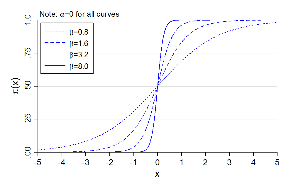
Smaller the slope, greater change in x required for a given change in Pr(y)

Probability curves with alpha = 0 and beta of 0.8, 1.6, 3.2, and 8.0: the larger beta, the steeper the S-curve.

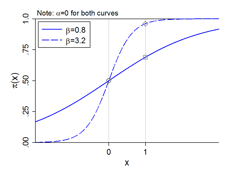
Changing β changes the effect of x

Probability curves with beta = 0.8 and beta = 3.2: the change in probability from x = 0 to x = 1 is much larger for the steeper curve.

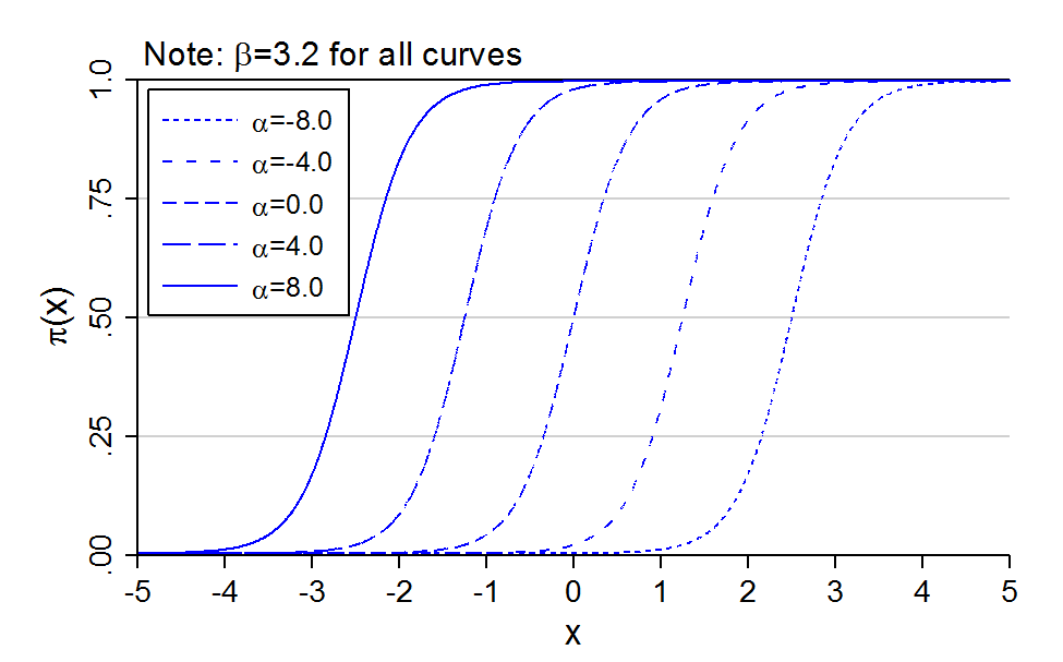
Changing the intercept

Smaller intercept, curve moves right

Probability curves with beta = 3.2 and alpha from -8 to 8: the S-curve keeps its shape and shifts right as alpha gets smaller.

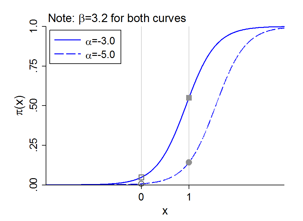
Changing α changes the effect of x

Probability curves with beta = 3.2 and alpha of -3 and -5: the change in probability from x = 0 to x = 1 differs between the two curves.

NOTE: This is why binary models are “inherently interactive.” Imagine the intercept shift (α) was due to a binary variable for college completion (=1). The effect of other variables (e.g., x could be age) are now automatically different for each group

Inherent interactions for continuous IVs

  • The same phenomenon of inherent interactions occurs for two continuous IVs
    • Consider two continuous IVs: x1 and x2
  • The intercept effectively absorbs the level of x2 causing an intercept shift
  • The model is:

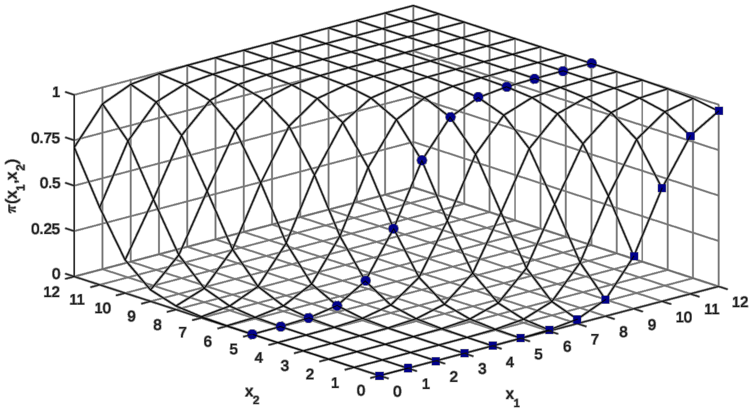
\[\Pr(y = 1\,|\,x_{1}, x_{2}) = \Phi(-4 + .6x_{1} + .5x_{2})\]

  • If x2=0 (curve with squares below):

\[\Pr(y = 1\,|\,x_{1}, x_{2} = 0) = \Phi(-4 + .6x_{1} + [.5 \times 0]) = \Phi(-4 + .6x_{1})\]

  • If x2=5 (curve with circles below):

\[\Pr(y = 1\,|\,x_{1}, x_{2} = 5) = \Phi(-4 + .6x_{1} + [.5 \times 5]) = \Phi([-4 + 2.5] + .6x_{1}) = {\color{blue}{\Phi(-1.5 + .6x_{1})}}\]

How x2 “affects the effect” of x1

Three-dimensional surface of the probability over x1 and x2: the curve for x2 = 0, marked with squares, and the curve for x2 = 5, marked with circles, rise at different values of x1.

Does the empirical relationship need to be S-shaped?

  • Does anyone in the sample need to have a probability near 0 or 1?
    • Can the relationship be relatively linear?
    • Can changes in x’s change the probability from 0 to 1 in the sample?

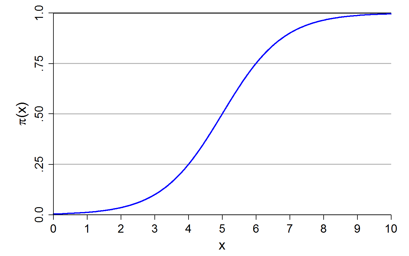
Where is your observed data located?

A full S-shaped probability curve from near 0 to near 1 as x goes from 0 to 10.

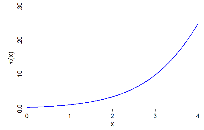
If only low or high probabilities are observed, very nonlinear

Only the bottom of the S-curve: probabilities from near 0 to 0.25, curving upward.

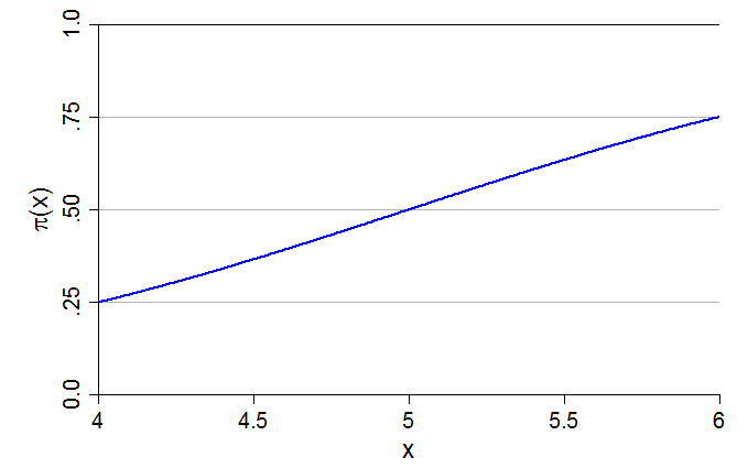
Change is mostly linear in middle of probability curve

Only the middle of the S-curve: probabilities from 0.25 to 0.75, close to a straight line.

Both of these are examples of just part of the logit probability curve being observed in the data (e.g., graph on left could be what you would observe for a rare outcome [i.e., few 1s on the DV]). Do you think the linear probability model (LPM) would predict similar probabilities? For one or the other? Both? Why?

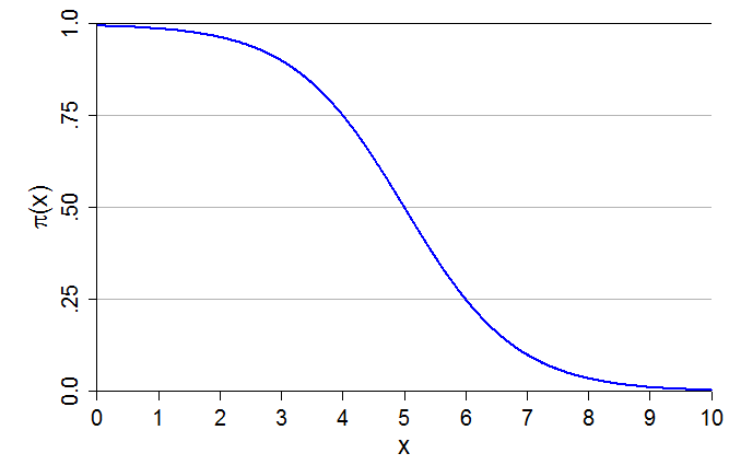
Negative relations are possible

A decreasing S-shaped probability curve from near 1 to near 0.

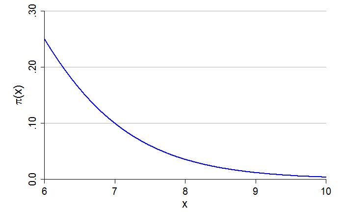
Only the bottom of a decreasing curve: probabilities falling from 0.25 toward 0.

And so on.

  • Note that these nonlinearities exist without any polynomials in the model for independent variables (e.g., x could be age—there is no x2 in our model)
    • See Appendix 3E for the effect of adding polynomial specifications of the IVs

GSS example: marijuana legalization

  • Let’s revisit our GSS example for support for legalizing marijuana use, but keep all available years (1975 to 2022)

Do you think the use of marijuana should be made legal or not?

use "https://tdmize.github.io/data/data/cda_gss22", clear
(GSS 1972-2022 CDA - Categorical Data Analysis | 2024-12-03)
drop if missing(grass, age, conserv, faminc, college, woman, race4)
(37,924 observations deleted)
recode grass 2 = 0
(0 changes made to grass)
lab def glab 0"not be legal" 1 "should be legal"
lab val grass glab
fre grass
grass -- should marijuana be made legal
-----------------------------------------------------------------------
                          |      Freq.    Percent      Valid       Cum.
--------------------------+--------------------------------------------
Valid   0 not be legal    |      21358      61.97      61.97      61.97
        1 should be legal |      13108      38.03      38.03     100.00
        Total             |      34466     100.00     100.00           
-----------------------------------------------------------------------
* Create year since 1975 variable
gen year1975 = year - 1975
lab var year1975 "years since 1975"
gss <- read_dta("https://tdmize.github.io/data/data/cda_gss22.dta")

# Drop any missing data on model vars
gss <- gss[complete.cases(gss[c("grass", "age", "conserv", "faminc", "college",
  "woman", "race4")]), ]
frq(gss, grass)
should marijuana be made legal (grass) <numeric> 
# total N=34466 valid N=34466 mean=0.38 sd=0.49

Value |           Label |     N | Raw % | Valid % | Cum. %
----------------------------------------------------------
    0 |    Not be legal | 21358 | 61.97 |   61.97 |  61.97
    1 | Should be legal | 13108 | 38.03 |   38.03 | 100.00
 <NA> |            <NA> |     0 |  0.00 |    <NA> |   <NA>
# Create year since 1975 variable
gss <- gss |> mutate(year1975 = as.numeric(year) - 1975)
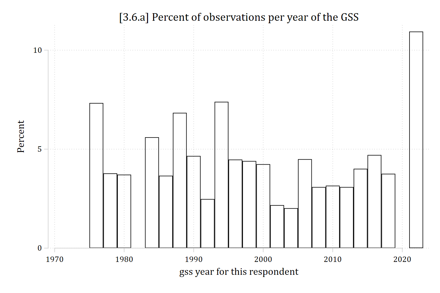
hist year if grass <= ., width(2) percent fcol(none) ///
    title("[3.6.a] Percent of observations per year of the GSS")
(bin=24, start=1975, width=2)

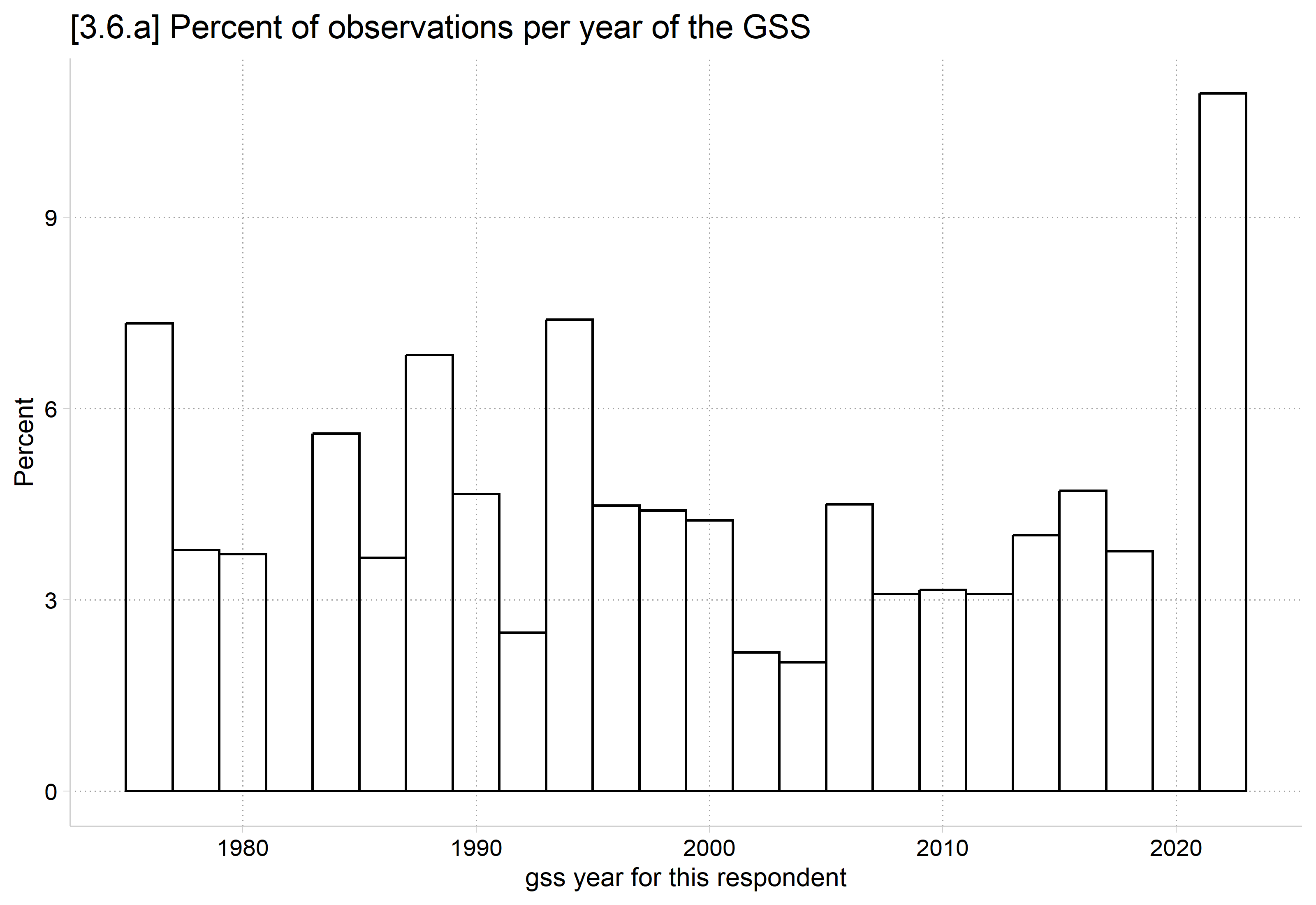
Histogram of the percent of observations in each two-year span of GSS years from 1975 to 2022: most spans have 2 to 7 percent, and the last span, 2021 to 2022, has about 11 percent.

ggplot(gss, aes(x = as.numeric(year))) +
  geom_histogram(aes(y = after_stat(100 * count / sum(count))),
    binwidth = 2, boundary = 1975, closed = "left", fill = NA, color = "black") +
  labs(title = "[3.6.a] Percent of observations per year of the GSS",
    x = "gss year for this respondent", y = "Percent")

Histogram of the percent of observations in each two-year span of GSS years from 1975 to 2022: most spans have 2 to 7 percent, and the last span, 2021 to 2022, has about 11 percent.

// binary logit model; or option for odds ratios
logit grass c.age c.year1975##c.year1975 i.conserv ///
    c.faminc i.degree i.woman i.race4, or
Iteration 0:  Log likelihood = -22892.973  
Iteration 1:  Log likelihood =  -19104.79  
Iteration 2:  Log likelihood =  -19063.87  
Iteration 3:  Log likelihood = -19063.784  
Iteration 4:  Log likelihood = -19063.784  

Logistic regression                                    Number of obs =  34,466
                                                       LR chi2(13)   = 7658.38
                                                       Prob > chi2   =  0.0000
Log likelihood = -19063.784                            Pseudo R2     =  0.1673

-------------------------------------------------------------------------------
        grass | Odds ratio   Std. err.      z    P>|z|     [95% conf. interval]
--------------+----------------------------------------------------------------
          age |      0.976      0.001  -29.637   0.000        0.975       0.978
     year1975 |      0.957      0.003  -12.883   0.000        0.951       0.964
              |
   c.year1975#|
   c.year1975 |      1.002      0.000   31.223   0.000        1.002       1.002
              |
      conserv |
Conservative  |      0.433      0.012  -30.040   0.000        0.410       0.457
       faminc |      0.999      0.000   -1.145   0.252        0.999       1.000
              |
       degree |
 high school  |      1.274      0.049    6.304   0.000        1.182       1.374
associate/..  |      1.435      0.085    6.079   0.000        1.277       1.612
  bachelor's  |      1.583      0.075    9.700   0.000        1.443       1.737
    graduate  |      1.782      0.102   10.080   0.000        1.593       1.994
              |
        woman |
       Women  |      0.669      0.017  -15.930   0.000        0.636       0.703
              |
        race4 |
       Black  |      0.856      0.033   -4.026   0.000        0.793       0.923
       Other  |      0.510      0.036   -9.554   0.000        0.445       0.586
    Hispanic  |      0.438      0.025  -14.631   0.000        0.392       0.489
              |
        _cons |      1.288      0.077    4.206   0.000        1.145       1.449
-------------------------------------------------------------------------------
Note: _cons estimates baseline odds.
est store mjmod
# Treat binary/nominal variables as factors using their value labels
gss <- gss |>
  mutate(conserv = as_factor(conserv), degree = as_factor(degree),
    woman = as_factor(woman), race4 = as_factor(race4)) |>
  droplevels()

mjmod <- glm(grass ~ age + poly(year1975, 2, raw = TRUE) + conserv + faminc + degree +
  woman + race4, data = gss, family = binomial(link = "logit"))

odds.ratio(mjmod, level = .95)
                                    OR   2.5 % 97.5 %         p    
(Intercept)                    1.28769 1.14448 1.4486 2.601e-05 ***
age                            0.97637 0.97482 0.9779 < 2.2e-16 ***
poly(year1975, 2, raw = TRUE)1 0.95739 0.95108 0.9638 < 2.2e-16 ***
poly(year1975, 2, raw = TRUE)2 1.00213 1.00199 1.0023 < 2.2e-16 ***
conservConservative            0.43256 0.40950 0.4568 < 2.2e-16 ***
faminc                         0.99948 0.99860 1.0004    0.2523    
degreehigh school              1.27404 1.18182 1.3739 2.903e-10 ***
degreeassociate/junior college 1.43519 1.27731 1.6124 1.209e-09 ***
degreebachelor's               1.58300 1.44281 1.7371 < 2.2e-16 ***
degreegraduate                 1.78223 1.59287 1.9943 < 2.2e-16 ***
womanWomen                     0.66873 0.63641 0.7027 < 2.2e-16 ***
race4Black                     0.85558 0.79290 0.9230 5.679e-05 ***
race4Other                     0.51031 0.44424 0.5855 < 2.2e-16 ***
race4Hispanic                  0.43812 0.39219 0.4892 < 2.2e-16 ***
---
Signif. codes:  0 '***' 0.001 '**' 0.01 '*' 0.05 '.' 0.1 ' ' 1

Odds ratio (OR) interpretations

Each additional year of age decreases the odds of supporting marijuana legalization by a factor of 0.98

Conservatives’ odds of supporting legalized marijuana are 0.43 times lower than non-conservatives

  • Are these large effects or small effects?
    • Do you have a sense of age’s effect size?
    • 0.43 is a large effect size in the odds metric (odds reduce more than half)
      • Can you guess how different the two groups are in terms of percentage points?
  • The year variable* shows significant linear and quadratic coefficients, but it is all but impossible to interpret its effect given the model is already nonlinear
  • To know substantive effect size, and to understand nonlinearities, must interpret in terms of predictions

*Variables with only very large values like year can cause problems. Solution: create a years since first observed year variable, here year1975 = year - 1975
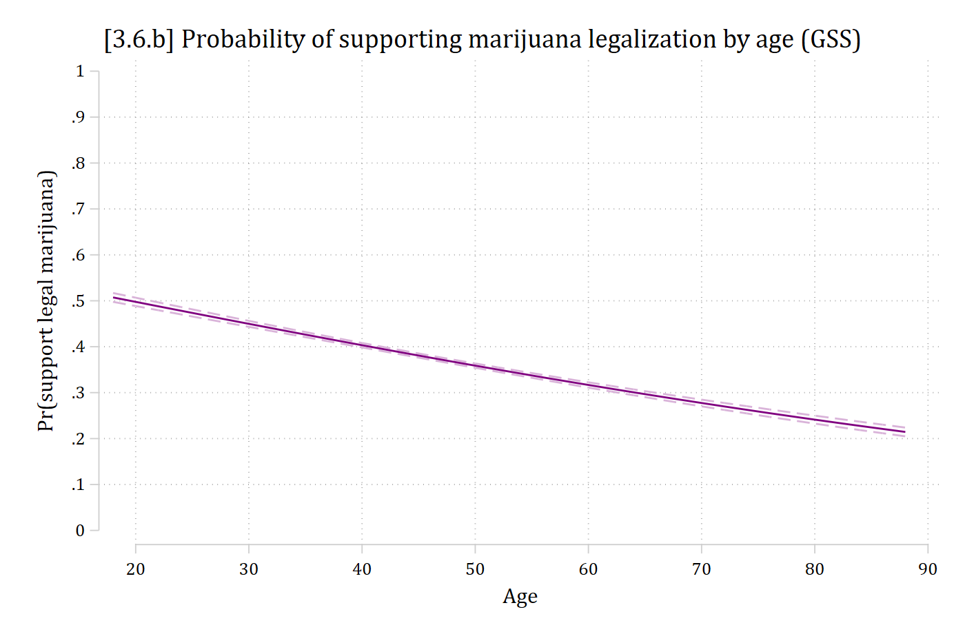
qui margins, at(age=(18(2)88))
marginsplot, ///
    plotop(msymbol(none) lcol(purple)) ///
    recastci(rline) ciopt(lpat(dash) lcol(purple*.3)) ///
    ylab(0(.1)1) ytitle("Pr(support legal marijuana)") xtitle("Age") ///
    xlab(20(10)90) ///
    title("[3.6.b] Probability of supporting marijuana legalization by age (GS
S)", size(*1.2))
Variables that uniquely identify margins: age

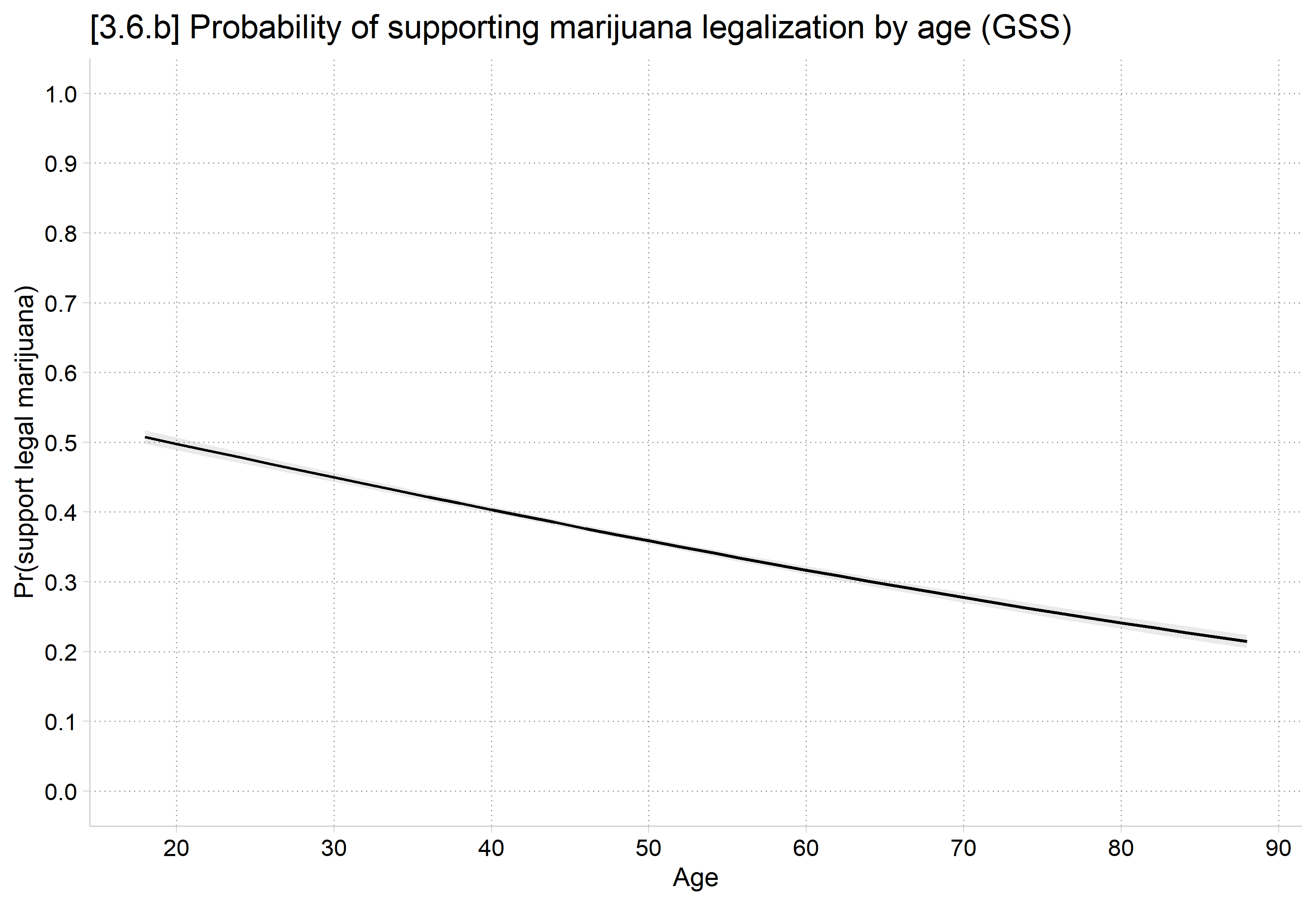
Predicted probability of supporting marijuana legalization by age: a nearly straight line falling from about 0.5 at age 18 to about 0.22 at age 88.

plot_predictions(mjmod, by = "age",
  newdata = datagrid(age = seq(18, 88, 2), grid_type = "counterfactual")) +
  scale_y_continuous(breaks = seq(0, 1, 0.1), limits = c(0, 1)) +
  scale_x_continuous(breaks = seq(20, 90, 10)) +
  labs(title = "[3.6.b] Probability of supporting marijuana legalization by age (GSS)",
    x = "Age", y = "Pr(support legal marijuana)")

Predicted probability of supporting marijuana legalization by age: a nearly straight line falling from about 0.5 at age 18 to about 0.22 at age 88.

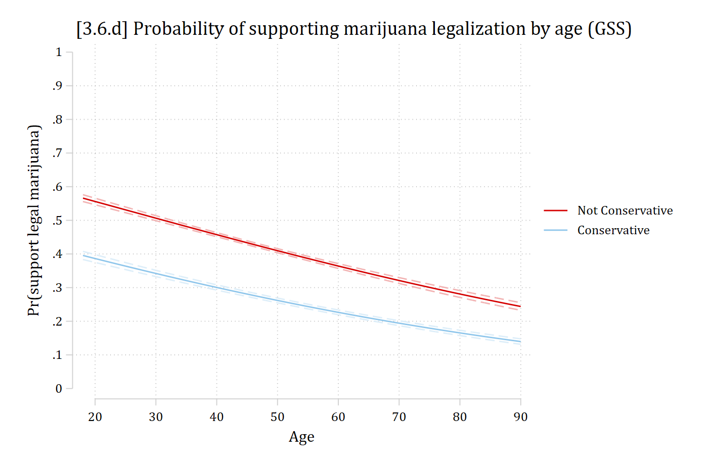
qui margins conserv, at(age=(18(2)90))
marginsplot, ///
    plotop(msymbol(none)) recastci(rline) ciopt(lpat(dash) lcol(*.3)) ///
    ylab(0(.1)1) ytitle("Pr(support legal marijuana)") xtitle("Age") ///
    xlab(20(10)90) ///
    title("[3.6.d] Probability of supporting marijuana legalization by age (GS
S)", size(*1.2))
Variables that uniquely identify margins: age conserv

Predicted probability of supporting marijuana legalization by age for non-conservatives and conservatives: both lines fall with age, and conservatives are lower at every age.

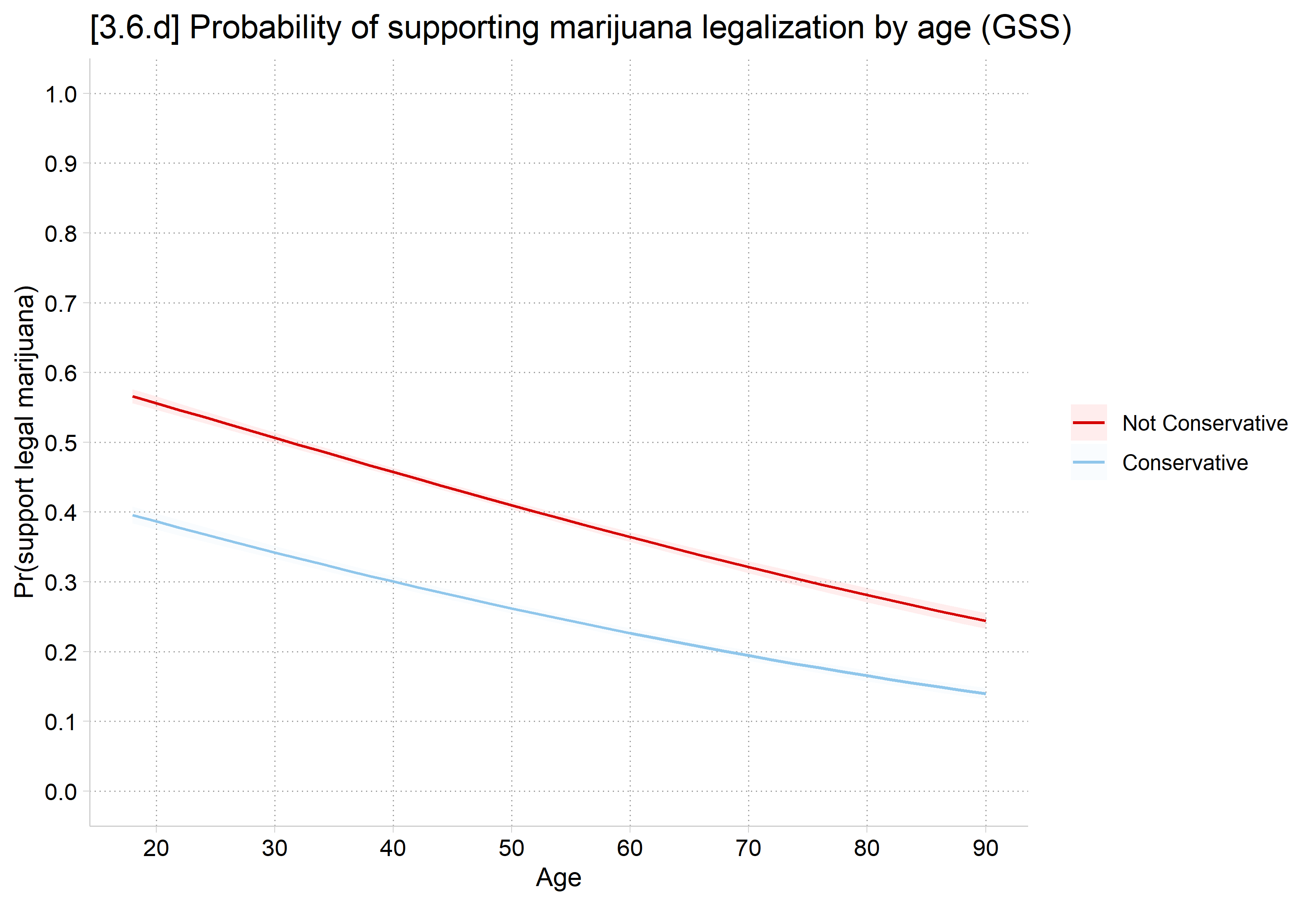
plot_predictions(mjmod, by = c("age", "conserv"),
  newdata = datagrid(age = seq(18, 90, 2), conserv = unique,
    grid_type = "counterfactual")) +
  scale_y_continuous(breaks = seq(0, 1, 0.1), limits = c(0, 1)) +
  scale_x_continuous(breaks = seq(20, 90, 10)) +
  labs(title = "[3.6.d] Probability of supporting marijuana legalization by age (GSS)",
    x = "Age", y = "Pr(support legal marijuana)", color = NULL, fill = NULL)

Predicted probability of supporting marijuana legalization by age for non-conservatives and conservatives: both lines fall with age, and conservatives are lower at every age.

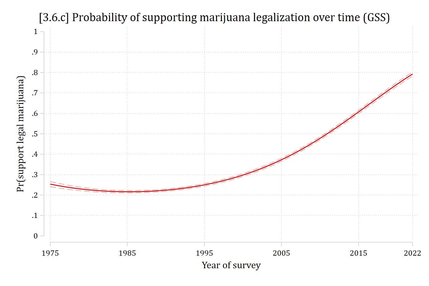
qui margins, at(year1975=(0(1)47))
marginsplot, ///
    plotop(msymbol(none)) recastci(rline) ciopt(lpat(dash) lcol(*.3)) ///
    ylab(0(.1)1) ytitle("Pr(support legal marijuana)") xtitle("Year of survey"
) ///
    xlab(0 "1975" 10 "1985" 20 "1995" 30 "2005" 40 "2015" 47 "2022") ///
    title("[3.6.c] Probability of supporting marijuana legalization over time 
(GSS)", size(*1.2))
Variables that uniquely identify margins: year1975

Predicted probability of supporting marijuana legalization by survey year: a U-shaped curve that dips slightly from 1975 to around 1990 and then rises steeply to about 0.8 in 2022.

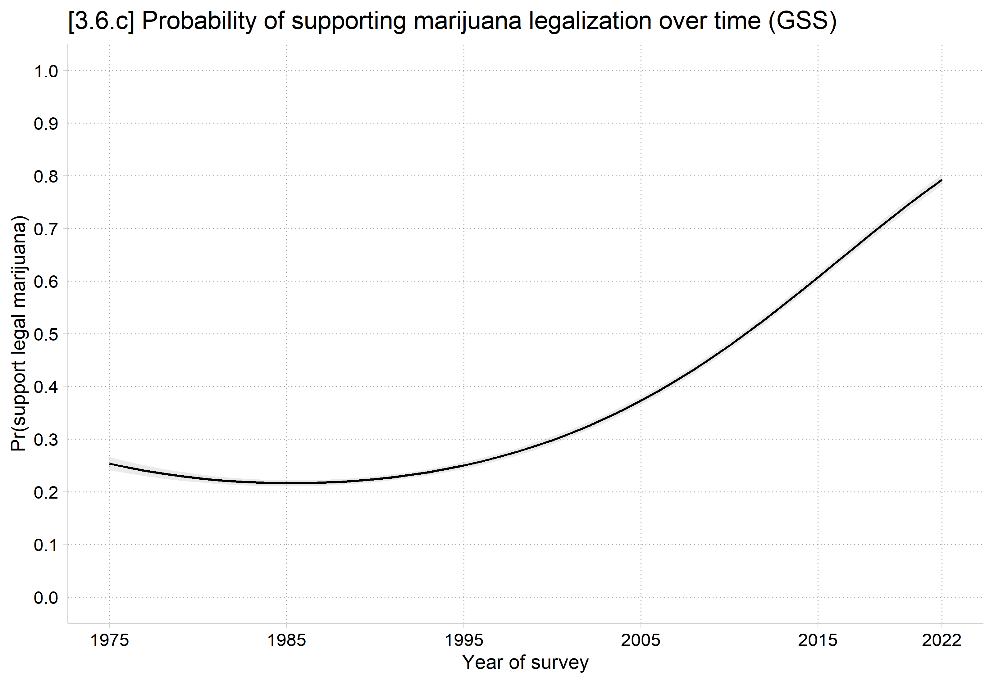
plot_predictions(mjmod, by = "year1975",
  newdata = datagrid(year1975 = 0:47, grid_type = "counterfactual")) +
  scale_y_continuous(breaks = seq(0, 1, 0.1), limits = c(0, 1)) +
  scale_x_continuous(breaks = c(0, 10, 20, 30, 40, 47),
    labels = c("1975", "1985", "1995", "2005", "2015", "2022")) +
  labs(title = "[3.6.c] Probability of supporting marijuana legalization over time (GSS)",
    x = "Year of survey", y = "Pr(support legal marijuana)")

Predicted probability of supporting marijuana legalization by survey year: a U-shaped curve that dips slightly from 1975 to around 1990 and then rises steeply to about 0.8 in 2022.

Back to top