7.7 Cross-Model Comparisons & Statistical Mediation

*Examples from Mize, Doan, and Long 2019

Overview of cross-model comparisons

  • I use the term cross-model comparisons as a general way to refer to comparing predictions and/or effects in one model to the predictions and/or effects in another model(s)
  • Statistical mediation is a common cross-model comparison; I use mediation* to illustrate the difficulties of comparing predictions/effects across categorical outcome models
    • The coefficients are not independently identified and “rescale” across models
      • The β coefficients cannot be compared directly across models
    • Predicted probabilities (and thus, marginal effects) are identified and do not rescale across models

*Note there is a growing body of work on causal mediation analysis I highly recommend learning more about (e.g., Imai et al. 2010; Keele 2015; Rudolph et al. 2018)

  • For the purposes of this class, I am showing the “traditional” approach often credited to Baron and Kenny 1986 JPSP. See Zhao, Lynch, and Chen 2010 for an excellent overview
  • The issues discussed here apply in both cases, and you can use MEs within the causal framework

Cross-model comparisons in linear vs nonlinear models

  • For linear models, can test the significance of a cross-model comparison as the difference in β coefficients across models
    • For mediation, this is identical to calculating the significance of the indirect effect
  • For nonlinear models, need a special approach to test for significant differences across multiple models. Two solutions:
    • Separate β coefficient into two parts:
      • Part representing explained variation (what you want)
      • Part representing model rescaling (a nuisance)
    • Combine multiple model estimates and compare marginal effects
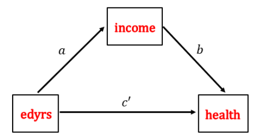
Mediation path diagram: edyrs has an arrow labeled a to income, income has an arrow labeled b to health, and a direct arrow labeled c-prime runs from edyrs to health.

Statistical mediation: the classic model

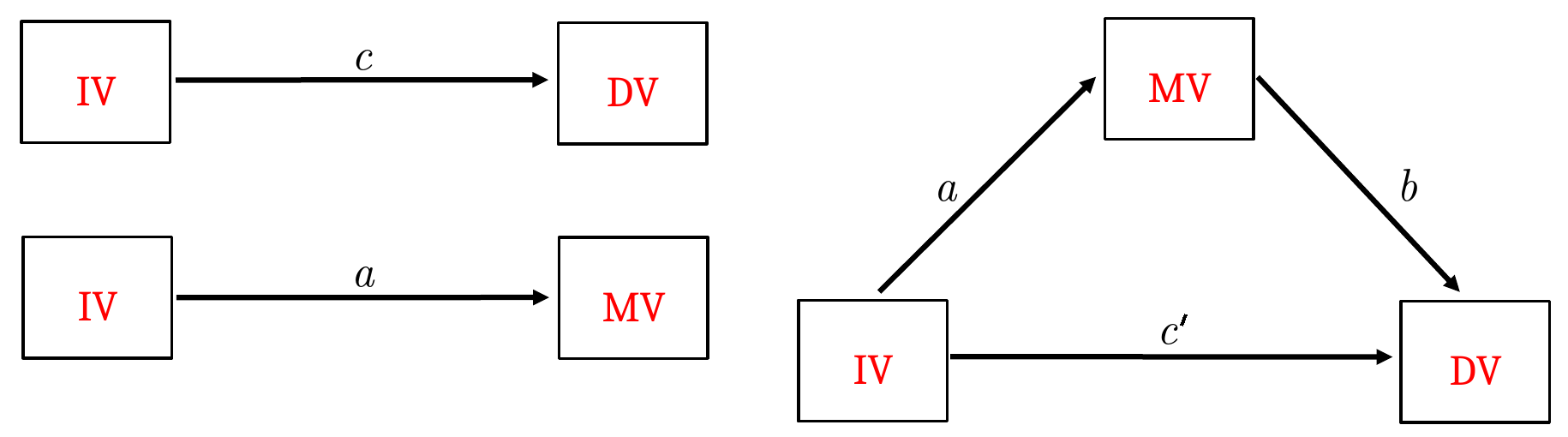
Three path diagrams. Top left: IV to DV, labeled c. Bottom left: IV to MV (the mediating variable), labeled a. Right: a triangle with IV to MV labeled a, MV to DV labeled b, and the direct path IV to DV labeled c-prime.

The mechanics of the tests are:

  1. First, regress the DV on the focal IV along with any control variables. The coefficient on the IV is c which represents the “total effect” on the IV (i.e., the effect before removing the portion of the effect explained by the mediator)
  2. Second, regress the mediating variable (MV) on the focal IV and control variables. The coefficient on the IV is path a.
  3. Third, regress the DV on the IV, the MV, and any control variables. The coefficient on the MV is path b. The coefficient on the IV is c’

Terminology for effects

  • Commonly, the effect of the IV before accounting for the mediator (c) is referred to as the total effect
  • The effect of the IV after accounting for the mediator (c’) is referred to as the direct effect
  • The difference in the total and direct effect is called the indirect effect—or the amount of the IV’s effect that is explained by the mediator

The test of mediation

  • Methodologists continue to debate what is needed to infer mediation*
    • The trend has been towards a single test \(a*b\) (or equivalently \(c - c'\)) needing to be significant and, if so, mediation is found
    • But, more recently, some have argued that if the a and the b path both are statistically significant there is mediation
  • I do both. I focus on the \(a*b = c - c'\) as my test of mediation, but estimate each individual model as described above to obtain a and b to understand the nature of mediation found (see Zhao et al. 2010 for details)

*E.g., See Preacher and Hayes 2004, Zhao et al. 2010, Yzerbyt et al. 2018

Statistical mediation and hypothesis testing

  • Many (most?) papers that test mediation do so informally
    • Commonly, researchers compare effects across models without directly testing the hypothesis of interest

“We get many submissions to the journal [ASR] attempting to test mediation… Authors usually proceed like this—they run one model with their key predictor plus controls and then a second model adding the mediator. If the coefficient of the key predictor is reduced or rendered nonsignificant, the authors conclude that the main effect has been mediated.” (Mustillo, Lizardo, and McVeigh 2018 ASR)

  • E.g., If the focal IV is significant at p < 0.05 in the first model but becomes p > 0.05 in the full model they interpret this as evidence of mediation
    • This is not a test of mediation

“There are several problems with this approach. Most commonly, authors fail to run a significance test for the difference in magnitude between coefficients. This step is necessary to determine whether mediation has occurred. The coefficient of the key predictor can be reduced or even rendered nonsignificant yet still be in the window of what could be considered to have occurred by chance alone… changes in statistical significance may not themselves be significant.” (Mustillo et al. 2018 ASR)

Direct tests of mediation

  1. We want to test whether the indirect effect is significant or can test whether effect of interest is significantly different in the two models

\[H_{0}: a*b = 0 \quad \textbf{or} \quad c - c' = 0\]

\[H_{A}: a*b \neq 0 \quad \textbf{or} \quad c - c' \neq 0\]

  1. This is different than a test of whether the effect is significant or not in each model
    • The significance test on the coefficient/ME is testing a different hypothesis

\[H_{0}: \beta = 0 \qquad H_{A}: \beta \neq 0\]

  1. Knowing whether an effect is significant or not in both models (as the hypothesis test in #2 above tests) is not a test of whether the effect has changed
    • E.g., Effect might be significant in both models, but still have a significant change across models
    • E.g., Effect might be significant in one model but not in the other, but still not have a significant change across models

Various SE formulas for test of a*b

  • The test of mediation is \(a*b\) (or equivalently \(c - c'\))

\[z = \frac{a*b}{\sqrt{a^{2}*\sigma_{b}^{2} + b^{2}*\sigma_{a}^{2} - \sigma_{a}^{2}*\sigma_{b}^{2}}}\]

  • In general, this test is usually referred to as the “Sobel test” or “Sobel-Goodman test” (see Sobel 1982 and Baron and Kenny 1986)
  • Results from different formulas for the tests tend to be similar
    • However, most have been found to be underpowered and alternative methods to calculate the standard error have been proposed. In particular, bootstrapping is a popular approach that has been shown to work well even in small samples (Preacher and Hayes 2004)

*NOTE: Showing the Sobel-Goodman approach to help you learn the logic of mediation. In practice, I recommend the SUEST + marginal effects approach shown later

Wald test to compare effects across models

  • A version of a Wald test can also be used in the context of testing predictions and/or effects across models and has better statistical properties than the traditional Sobel-Goodman tests because it accounts for the covariance between the effects (Mize, Doan, and Long 2019)
    • In the case of mediation, to test if \(c = c'\)

\[z = \frac{c - c'}{\sqrt{\sigma_{c}^{2} + \sigma_{c'}^{2} - 2(\sigma_{c,c'})}}\]

  • Where \(\sigma_{c}^{2}\) is the variance of the estimate (\(\sqrt{\sigma_{c}^{2}}\) is the standard error)
    • And \(\sigma_{c,c'}\) is the covariance between the two effects*

*The covariance is the difficult part to estimate, but a very important one—more on this in Section 7.9

Statistical mediation: linear regression example

  • Example: Add Health Wave 4
    • DV: depressive symptoms
    • Focal IV: education in years
    • Mediating IV: wages
*Sobel Test Example
use "https://tdmize.github.io/data/data/addhealth4", clear
(addhealth4_dmv.dta | Add Health Wave IV | DMV Workshop)
regress depscale c.edyrs
      Source |       SS           df       MS      Number of obs   =     4,307
-------------+----------------------------------   F(1, 4305)      =    108.52
       Model |  22.0288344         1  22.0288344   Prob > F        =    0.0000
    Residual |   873.92287     4,305  .203001828   R-squared       =    0.0246
-------------+----------------------------------   Adj R-squared   =    0.0244
       Total |  895.951704     4,306   .20807053   Root MSE        =    .45056

------------------------------------------------------------------------------
    depscale | Coefficient  Std. err.      t    P>|t|     [95% conf. interval]
-------------+----------------------------------------------------------------
       edyrs |     -0.032      0.003  -10.417   0.000       -0.038      -0.026
       _cons |      1.043      0.045   23.340   0.000        0.956       1.131
------------------------------------------------------------------------------
regress depscale c.edyrs c.wages
      Source |       SS           df       MS      Number of obs   =     4,307
-------------+----------------------------------   F(2, 4304)      =     68.58
       Model |  27.6703625         2  13.8351812   Prob > F        =    0.0000
    Residual |  868.281342     4,304   .20173823   R-squared       =    0.0309
-------------+----------------------------------   Adj R-squared   =    0.0304
       Total |  895.951704     4,306   .20807053   Root MSE        =    .44915

------------------------------------------------------------------------------
    depscale | Coefficient  Std. err.      t    P>|t|     [95% conf. interval]
-------------+----------------------------------------------------------------
       edyrs |     -0.029      0.003   -9.309   0.000       -0.035      -0.023
       wages |     -0.002      0.000   -5.288   0.000       -0.002      -0.001
       _cons |      1.029      0.045   23.053   0.000        0.941       1.116
------------------------------------------------------------------------------
library(haven)           # import Stata data and labels
library(modelsummary)    # regression tables

ah4 <- read_dta("https://tdmize.github.io/data/data/addhealth4.dta")

# Sobel Test Example
total <- lm(depscale ~ edyrs, data = ah4)
direct <- lm(depscale ~ edyrs + wages, data = ah4)

modelsummary(list(total, direct), fmt = 3,
  stars = c("*" = .05, "**" = .01, "***" = .001))
(1) (2)
* p < 0.05, ** p < 0.01, *** p < 0.001
(Intercept) 1.043*** 1.029***
(0.045) (0.045)
edyrs -0.032*** -0.029***
(0.003) (0.003)
wages -0.002***
(0.000)
Num.Obs. 4307 4307
R2 0.025 0.031
R2 Adj. 0.024 0.030
AIC 5359.1 5333.2
BIC 5378.2 5358.6
Log.Lik. -2676.526 -2662.579
F 108.515 68.580
RMSE 0.45 0.45
  • Effect size reduced from -0.032 to -0.029 (change of 0.003). Sometimes useful to discuss this in terms of the proportion reduction in the effect:

Proportion reduction in effect of focal IV due to mediating variable (MV):

\[\frac{a*b}{c} = \frac{c - c'}{c} = 1 - \frac{c'}{c}\]

di 1 - (-0.029 / -0.032)
.09375
1 - (-0.029 / -0.032)
[1] 0.09375

The effect of education is reduced by about 9% after accounting for wages

  • However, we have not yet tested whether this is a significant reduction in the effect
  • In Stata, my command sgmediation2 will estimate each of the individual models and estimate the test of the indirect effect for you
sgmediation2 depscale, mv(wages) iv(edyrs)
Model with dv regressed on iv (path c)
 regress depscale edyrs , vce() 

      Source |       SS           df       MS      Number of obs   =     4,307
-------------+----------------------------------   F(1, 4305)      =    108.52
       Model |  22.0288344         1  22.0288344   Prob > F        =    0.0000
    Residual |   873.92287     4,305  .203001828   R-squared       =    0.0246
-------------+----------------------------------   Adj R-squared   =    0.0244
       Total |  895.951704     4,306   .20807053   Root MSE        =    .45056

------------------------------------------------------------------------------
    depscale | Coefficient  Std. err.      t    P>|t|     [95% conf. interval]
-------------+----------------------------------------------------------------
       edyrs |     -0.032      0.003  -10.417   0.000       -0.038      -0.026
       _cons |      1.043      0.045   23.340   0.000        0.956       1.131
------------------------------------------------------------------------------

Model with mediator regressed on iv (path a)
 regress wages edyrs , vce() 

      Source |       SS           df       MS      Number of obs   =     4,307
-------------+----------------------------------   F(1, 4305)      =    148.22
       Model |  74140.5856         1  74140.5856   Prob > F        =    0.0000
    Residual |  2153341.01     4,305  500.195357   R-squared       =    0.0333
-------------+----------------------------------   Adj R-squared   =    0.0331
       Total |   2227481.6     4,306  517.297166   Root MSE        =    22.365

------------------------------------------------------------------------------
       wages | Coefficient  Std. err.      t    P>|t|     [95% conf. interval]
-------------+----------------------------------------------------------------
       edyrs |      1.845      0.152   12.175   0.000        1.548       2.142
       _cons |     -8.770      2.218   -3.953   0.000      -13.120      -4.421
------------------------------------------------------------------------------

Model with dv regressed on mediator and iv (paths b and c')
 regress depscale wages edyrs , vce() 

      Source |       SS           df       MS      Number of obs   =     4,307
-------------+----------------------------------   F(2, 4304)      =     68.58
       Model |  27.6703625         2  13.8351812   Prob > F        =    0.0000
    Residual |  868.281342     4,304   .20173823   R-squared       =    0.0309
-------------+----------------------------------   Adj R-squared   =    0.0304
       Total |  895.951704     4,306   .20807053   Root MSE        =    .44915

------------------------------------------------------------------------------
    depscale | Coefficient  Std. err.      t    P>|t|     [95% conf. interval]
-------------+----------------------------------------------------------------
       wages |     -0.002      0.000   -5.288   0.000       -0.002      -0.001
       edyrs |     -0.029      0.003   -9.309   0.000       -0.035      -0.023
       _cons |      1.029      0.045   23.053   0.000        0.941       1.116
------------------------------------------------------------------------------

Sobel-Goodman Mediation Tests

                     |        Est     Std_err           z       P>|z| 
---------------------+-----------------------------------------------
               Sobel |     -0.003       0.001      -4.850       0.000 
              Aroian |     -0.003       0.001      -4.837       0.000 
             Goodman |     -0.003       0.001      -4.864       0.000 

Indirect, Direct, and Total Effects

                     |        Est     Std_err           z       P>|z| 
---------------------+-----------------------------------------------
       a_coefficient |      1.845       0.152      12.175       0.000 
       b_coefficient |     -0.002       0.000      -5.288       0.000 
 Indirect_effect_aXb |     -0.003       0.001      -4.850       0.000 
    Direct_effect_c' |     -0.029       0.003      -9.309       0.000 
      Total_effect_c |     -0.032       0.003     -10.417       0.000 


Proportion of total effect that is mediated:       0.094
Ratio of indirect to direct effect:                0.104
Ratio of total to direct effect:                   1.104
# R has no built-in way to do the Sobel-Goodman tests that sgmediation2 reports,
# so estimate each path and calculate the tests by hand
apath <- lm(wages ~ edyrs, data = ah4)       # path a
# total (path c) and direct (paths b and c') were fit above

a <- coef(apath)[["edyrs"]];   sa <- sqrt(vcov(apath)["edyrs", "edyrs"])
b <- coef(direct)[["wages"]];  sb <- sqrt(vcov(direct)["wages", "wages"])
tot <- coef(total)[["edyrs"]]; stot <- sqrt(vcov(total)["edyrs", "edyrs"])
dir <- tot - a * b;            sdir <- sqrt(vcov(direct)["edyrs", "edyrs"])

ztest <- function(est, se) {
  z <- est / se
  round(c(Est = est, Std_err = se, z = z, "P>|z|" = 2 * pnorm(-abs(z))), 3)
}

# Sobel-Goodman Mediation Tests
rbind(Sobel   = ztest(a * b, sqrt(b^2 * sa^2 + a^2 * sb^2)),
      Aroian  = ztest(a * b, sqrt(b^2 * sa^2 + a^2 * sb^2 + sa^2 * sb^2)),
      Goodman = ztest(a * b, sqrt(b^2 * sa^2 + a^2 * sb^2 - sa^2 * sb^2)))
           Est Std_err      z P>|z|
Sobel   -0.003   0.001 -4.850     0
Aroian  -0.003   0.001 -4.837     0
Goodman -0.003   0.001 -4.864     0
# Indirect, Direct, and Total Effects
rbind(a_coefficient = ztest(a, sa),
      b_coefficient = ztest(b, sb),
      Indirect_effect_aXb = ztest(a * b, sqrt(b^2 * sa^2 + a^2 * sb^2)),
      "Direct_effect_c'" = ztest(dir, sdir),
      Total_effect_c = ztest(tot, stot))
                       Est Std_err       z P>|z|
a_coefficient        1.845   0.152  12.175     0
b_coefficient       -0.002   0.000  -5.288     0
Indirect_effect_aXb -0.003   0.001  -4.850     0
Direct_effect_c'    -0.029   0.003  -9.309     0
Total_effect_c      -0.032   0.003 -10.417     0
# Proportion of total effect that is mediated; ratios of indirect to direct
# and of total to direct effect
round(c(Proportion_mediated = a * b / tot, Indirect_to_direct = a * b / dir,
  Total_to_direct = tot / dir), 3)
Proportion_mediated  Indirect_to_direct     Total_to_direct 
              0.094               0.104               1.104 

Interpretations below…

Interpreting mediation

Focusing on the a*b (c – c’) test:

Education’s effect on depressive symptoms is partially mediated by the effect of wages. The effect of education is reduced by about 9% after accounting for the effect of wages (p < 0.001)

Alternatively, focusing on the a and b paths:

More education is associated with higher wages (a path p < 0.001). In turn, higher wages are associated with fewer depressive symptoms (b path p < 0.001). Taken together, this suggests that wages mediate the relationship between education and depressive symptoms.

Example presentation of mediation results

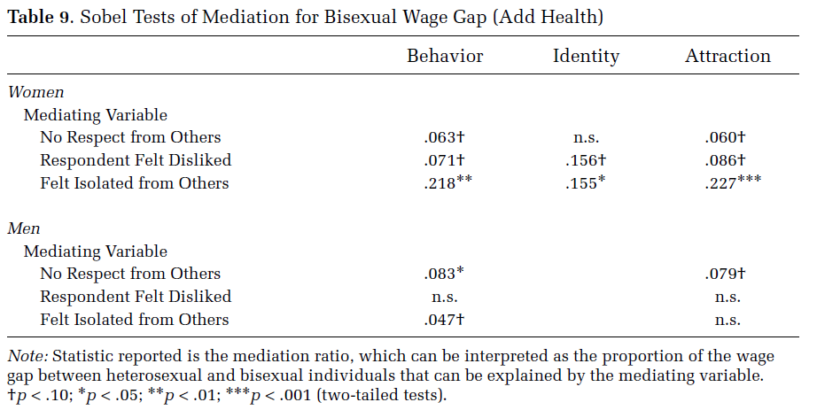
Table 9 from Mize (2016): Sobel tests of mediation for the bisexual wage gap in Add Health, separately for women and men. Columns are behavior, identity, and attraction; rows are mediating variables (no respect from others, respondent felt disliked, felt isolated from others), with mediation ratios such as .218** for women's isolation under behavior and n.s. where not significant.

*Table from Mize 2016

Back to top