A2.10 Transforming variables

• There are an almost unlimited number of ways you can transform your variables to alter their distribution
  • A non-normal DV is a common rationale for transformation. Note that this is not necessary (linear regression does not require normally distributed DVs)—but can be helpful when the mean does not summarize the distribution well
  • Non-normal IVs are not necessarily problematic—though outliers can influence effects
    • Large confidence intervals will appropriately reflect places in data with few cases
• The Stata command gladder is helpful to quickly visualize what various transformations would look like
  • This is based on Tukey’s (1977) ladder of powers which provides an empirical way to determine whether a transformation will normalize the distribution of a continuous variable
  • With large datasets, the statistical tests for this become all but meaningless—I prefer looking at it visually

use "https://tdmize.github.io/data/data/gss", clear

(gss.dta | GSS 1972 - 2016 Data | DMV Workshop)

gladder wages, title("[2.5.e] Distributions of Various Transformations of Wage
s")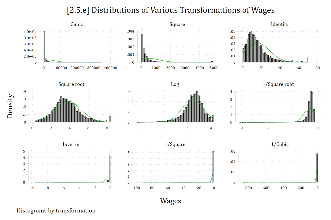

use "https://tdmize.github.io/data/data/cda_ah4", clear

(cda_ah4.dta | Add Health Wave 4 - | )

clonevar exercisSS2 = exercisSS

(5 missing values generated)

replace exercisSS2 = exercisSS2 + 1

(5,109 real changes made)

gladder exercisSS2, title("[2.5.f] Distributions of Various Transformations") 
///
    subtitle("Activity Scale: Times Active in Last Week")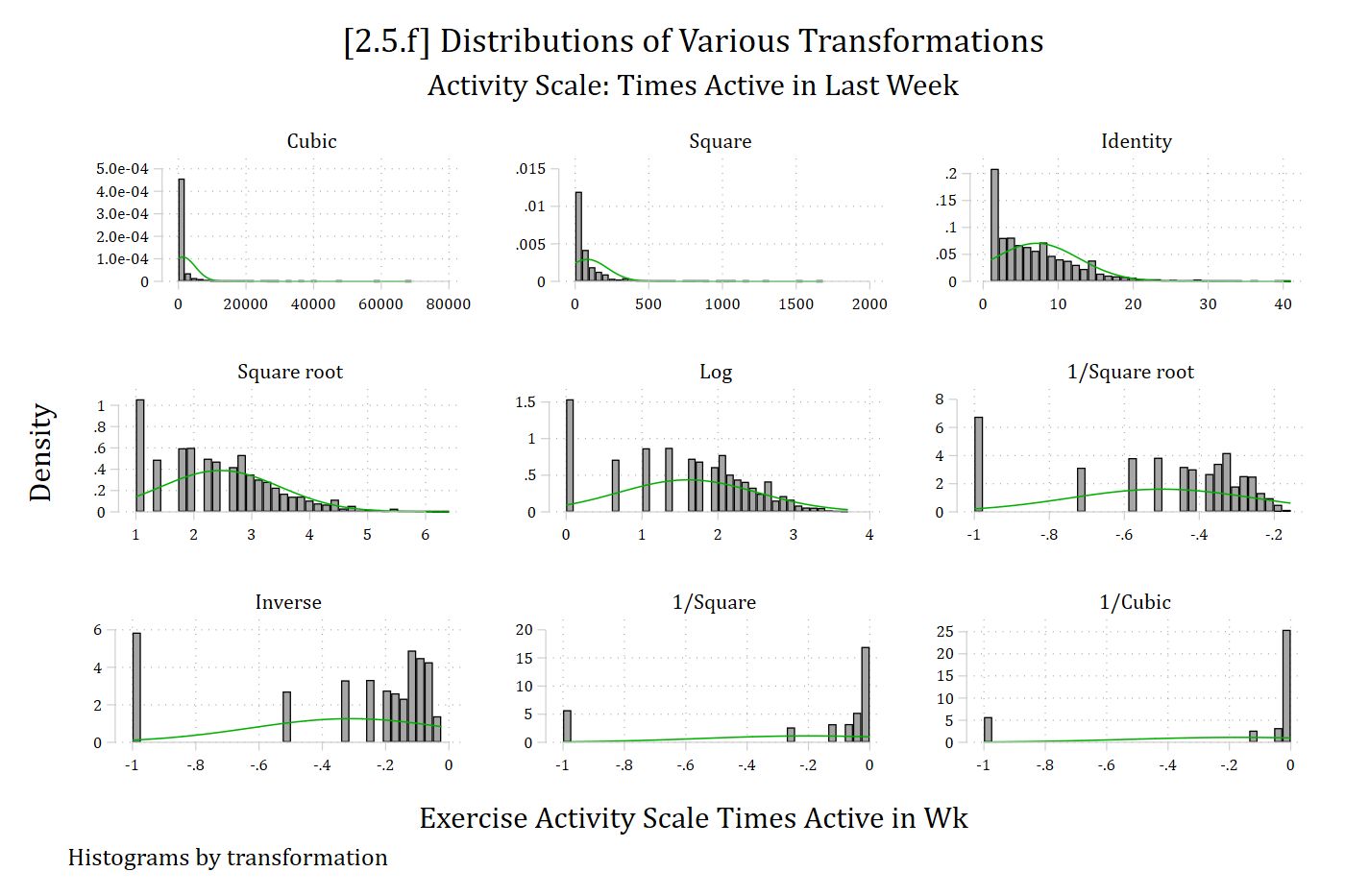

*None of the transformations do a great job for this variable—largely because there is a large peak at zero (the modal person reports no physical activity). The best way to deal with this variable as a DV would be a count model (more on that later in the semester!)