2. Use graph types people read accurately

  • Pie charts, bar charts, and dot plots can often display the same information: usually, the univariate distribution of a categorical variable
    • But, most can also be used for bivariate relationships and we will use these as building blocks for visualizing more complicated relationships
  • Despite their similarities, they can differ dramatically in their effectiveness

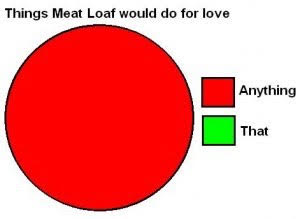
Joke pie chart titled Things Meat Loaf would do for love: the whole pie is Anything and none of it is That.

Meatloaf music video (highly recommended)

Pie charts

  • Pie charts present the proportion of a variable represented in each category
    • The fundamental rule of a pie chart is it should show parts of a whole
    • E.g., Among the Purdue student population, what percent major in engineering, social science, health/medical fields, humanities, etc.?

A crowd of Purdue students with the Purdue Pete mascot.

  • Pie charts have the advantage of being intuitive to understand and widely used—so your audience is probably familiar with them
  • The downside of a pie chart is that judging area size and angles is hard
    • The reader receives more of a general sense of the size of different categories rather than a precise estimate
    • There are no axis labels that can be referred to
use "https://tdmize.github.io/data/data/hrs_si.dta", clear
(Health and Retirement Study 1992-2022 - Cleaned for MCAP SI)
// 2.a - Pie charts are generally not recommended
graph pie, over(srhealth) ///
    title("[2.a] Pie chart for distribution of self-rated health among older a
dults")

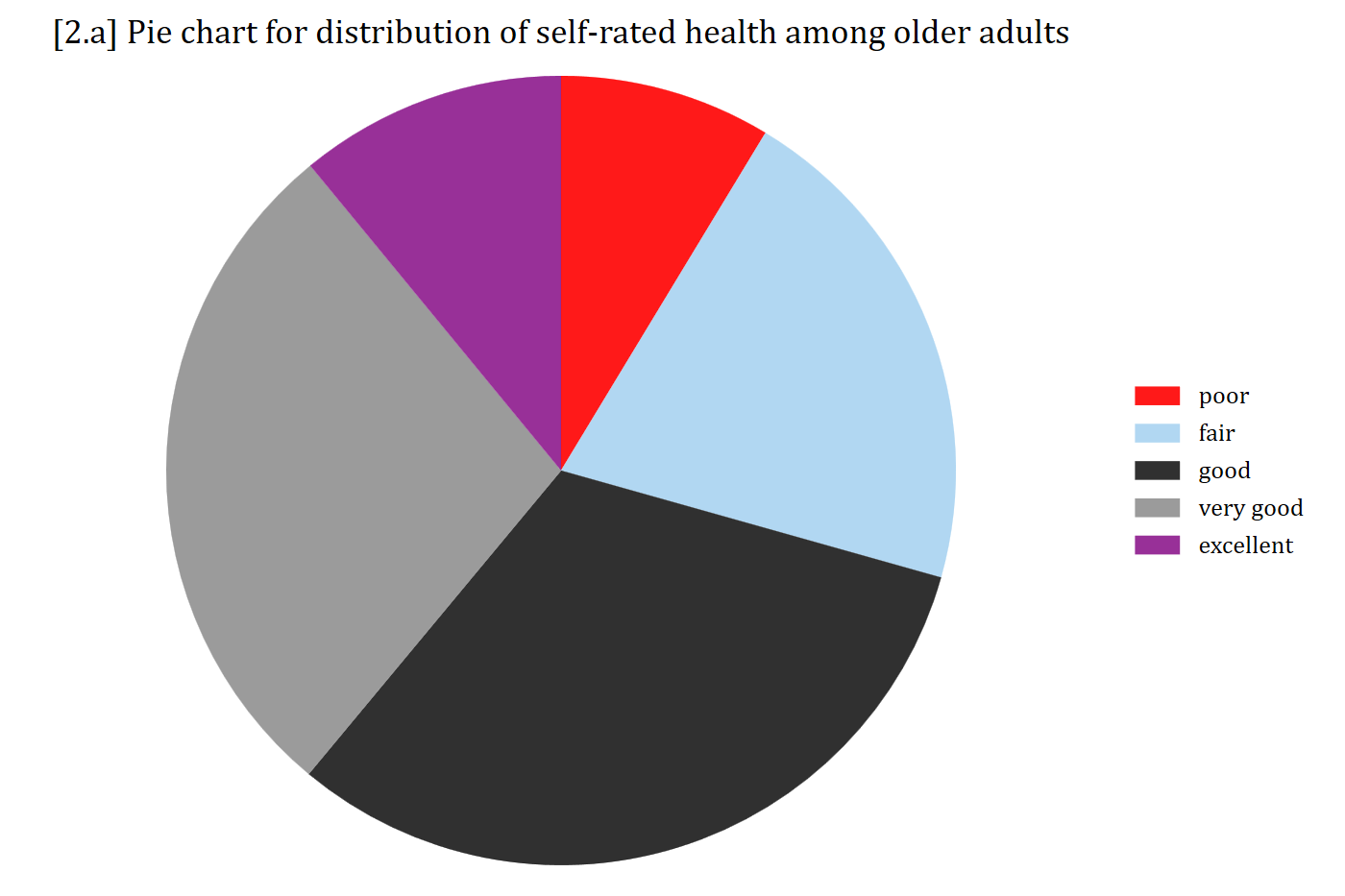
[2.a] Pie chart of self-rated health among older adults with five slices (poor, fair, good, very good, excellent): good and very good are the largest slices, but the sizes of the slices are hard to compare precisely.

library(foreign)            # load Stata datasets
library(ggplot2)            # main graphics package
library(dplyr)              # data manipulation tools
library(cleanplots)         # Mize's graphics scheme

## Use cleanplots colors, markers, lines, and theme for all graphs ##
cleanplots_defaults()
theme_update(plot.title.position = "plot")   # titles start at left edge of graph

# Health and Retirement Study Data
hrs <- read.dta("https://tdmize.github.io/data/data/hrs_si.dta")

# 2.a - Pie charts (generally not recommended)
ggplot(filter(hrs, !is.na(srhealth)), aes(x = "", fill = srhealth)) +
  geom_bar(width = 1) +
  coord_polar(theta = "y") +
  labs(title = "[2.a] Pie chart for distribution of self-rated health among older adults",
       fill = "") +
  scale_fill_viridis_d() +
  theme_void(base_size = 12)

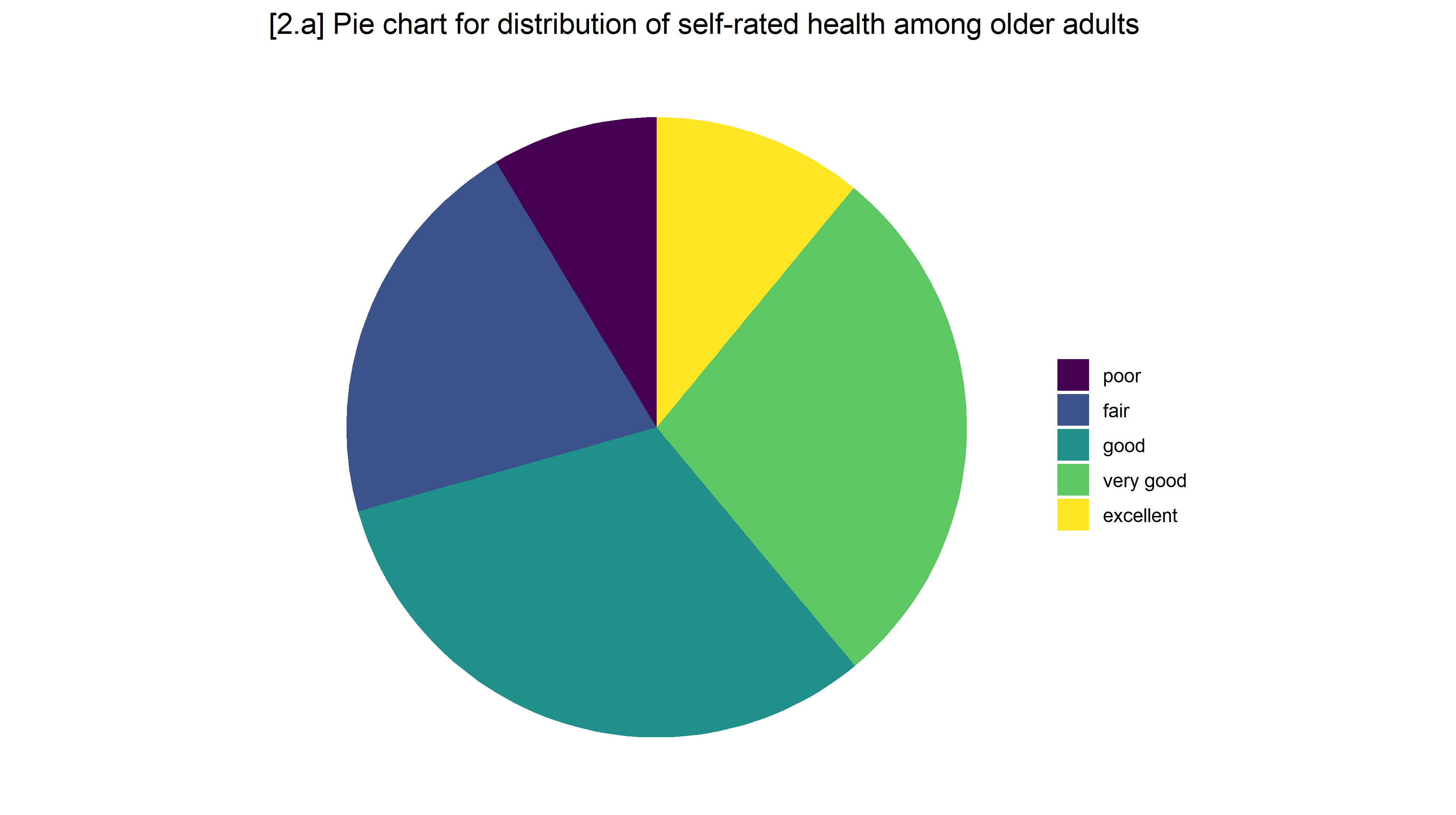
[2.a] Pie chart of self-rated health among older adults with five slices (poor, fair, good, very good, excellent): good and very good are the largest slices, but the sizes of the slices are hard to compare precisely.

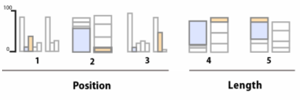
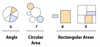
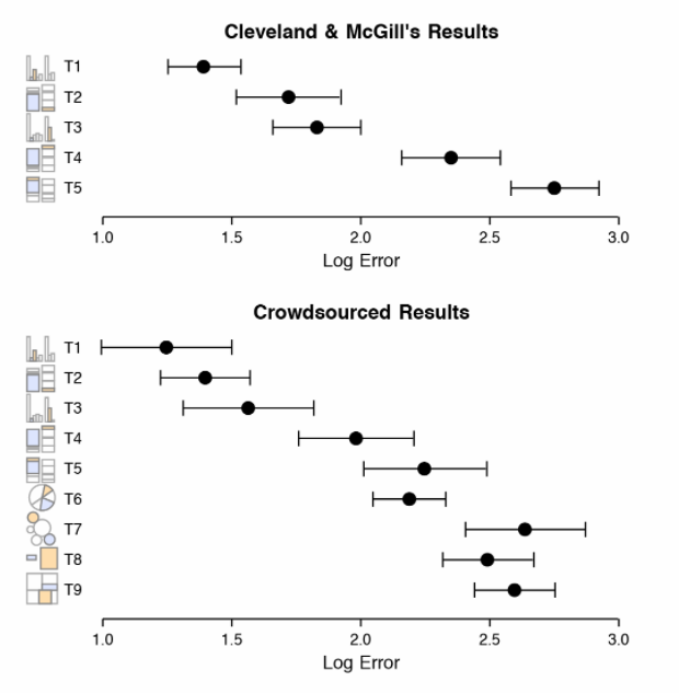
Accuracy of perceptual tasks

Dot plots of the log error for each task, in Cleveland and McGill's results and in crowdsourced results: errors are smallest for judging position and length and largest for angles and areas.

Note: “crowdsourced” results refer to Heer & Bostock (2010)

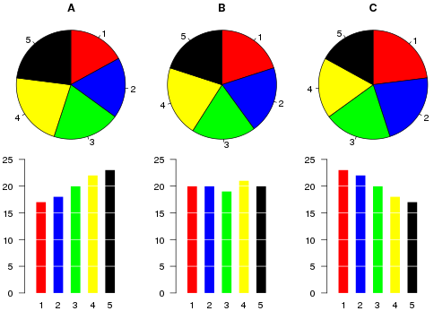
Three pie charts (A, B, C) with five similar-sized slices each, above bar charts of the same data: the differences between the categories are hard to see in the pies and easy to see in the bars.

*Bar charts are simple but very effective for comparing amounts across groups

Stacked bar charts

  • Stacked bar charts are a useful alternative to pie charts
    • Also, make it easy to compare across time/waves or groups (which is very difficult with a pie chart)
  • Stacked bar charts can be used when you want a bar to fill the entire space of an axis (compare to how much space on the y-axis is covered by the bars above)
  • Stacked bar charts are especially useful when you have categorical outcome (y) variables and/or when the total of multiple variables is of interest
    • Works well for binary dependent variables
    • Especially useful for nominal/ordinal dependent variables
* Create variable to flag cohort of respondents who were in first wave of data
egen byte in1992 = max(year == 1992), by(hhidpn)
tab in1992
     in1992 |      Freq.     Percent        Cum.
------------+-----------------------------------
          0 |    171,820       58.01       58.01
          1 |    124,377       41.99      100.00
------------+-----------------------------------
      Total |    296,197      100.00
// 2.b - Stacked bar chart
graph bar (count) if in1992, ///
    over(srhealth) horizontal asyvars stack percentages ///
    ytitle("Self-rated health") title("") ///
    scheme(cleanplots5) legen(pos(6) row(1)) xsize(8) ysize(2) scale(2.5)

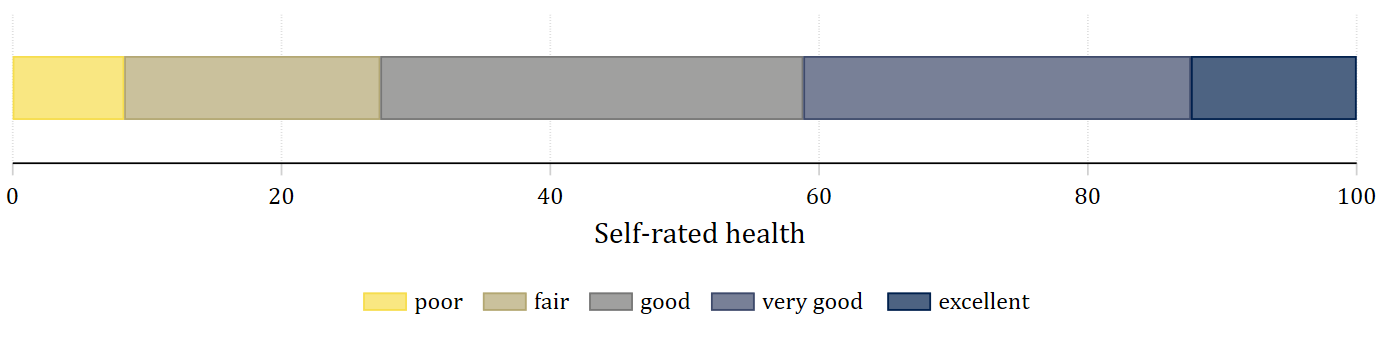
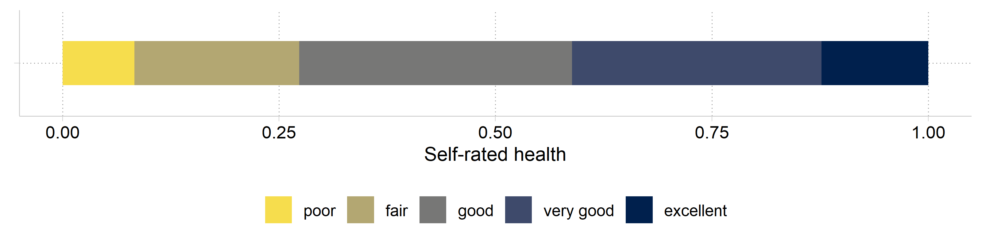
[2.b] A single horizontal stacked bar of self-rated health from 0 to 100 percent, in ordinal colors from light yellow (poor) to dark blue (excellent): about 8% poor, 19% fair, 31% good, 29% very good, and 12% excellent.

# Quick work to flag only those included in first HRS wave
ids_1992 <- hrs %>%
  filter(year == 1992) %>%
  pull(hhidpn) %>% unique()

hrs_filtered <- hrs %>%
  filter(hhidpn %in% ids_1992)

# 2.b - Stacked bar chart
ggplot(filter(hrs_filtered, !is.na(srhealth)), aes(y = "", fill = srhealth)) +
  geom_bar(position = position_fill(reverse = TRUE), width = .5) +
  labs(x = "Self-rated health", y = NULL, fill = "") +
  scale_fill_viridis_d(option = "cividis", direction = -1, end = .95) +
  theme(legend.position = "bottom")

[2.b] A single horizontal stacked bar of self-rated health from 0 to 100 percent, in ordinal colors from light yellow (poor) to dark blue (excellent): about 8% poor, 19% fair, 31% good, 29% very good, and 12% excellent.

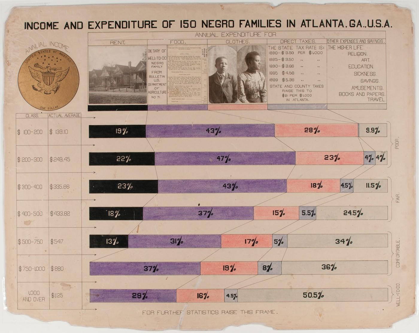
Historical example: W.E.B DuBois

W.E.B. Du Bois's hand-drawn chart Income and Expenditure of 150 Negro Families in Atlanta, GA., U.S.A.: stacked horizontal bars showing how each income group spent its money.

*Read more about W.E.B. DuBois’s pioneering data visualizations here (and a whole book here)

// 2.c - Stacked bar chart with 1992 cohort: ordinal colors from cleanplots5 s
cheme
graph bar (count) if in1992, ///
    over(srhealth) over(year) ///
    asyvars stack percentages ///
    ytitle("Self-rated health") ///
    title("[2.c] Stacked bar chart of self-rated health among older adults ove
r time (HRS)") ///
    scheme(cleanplots5)

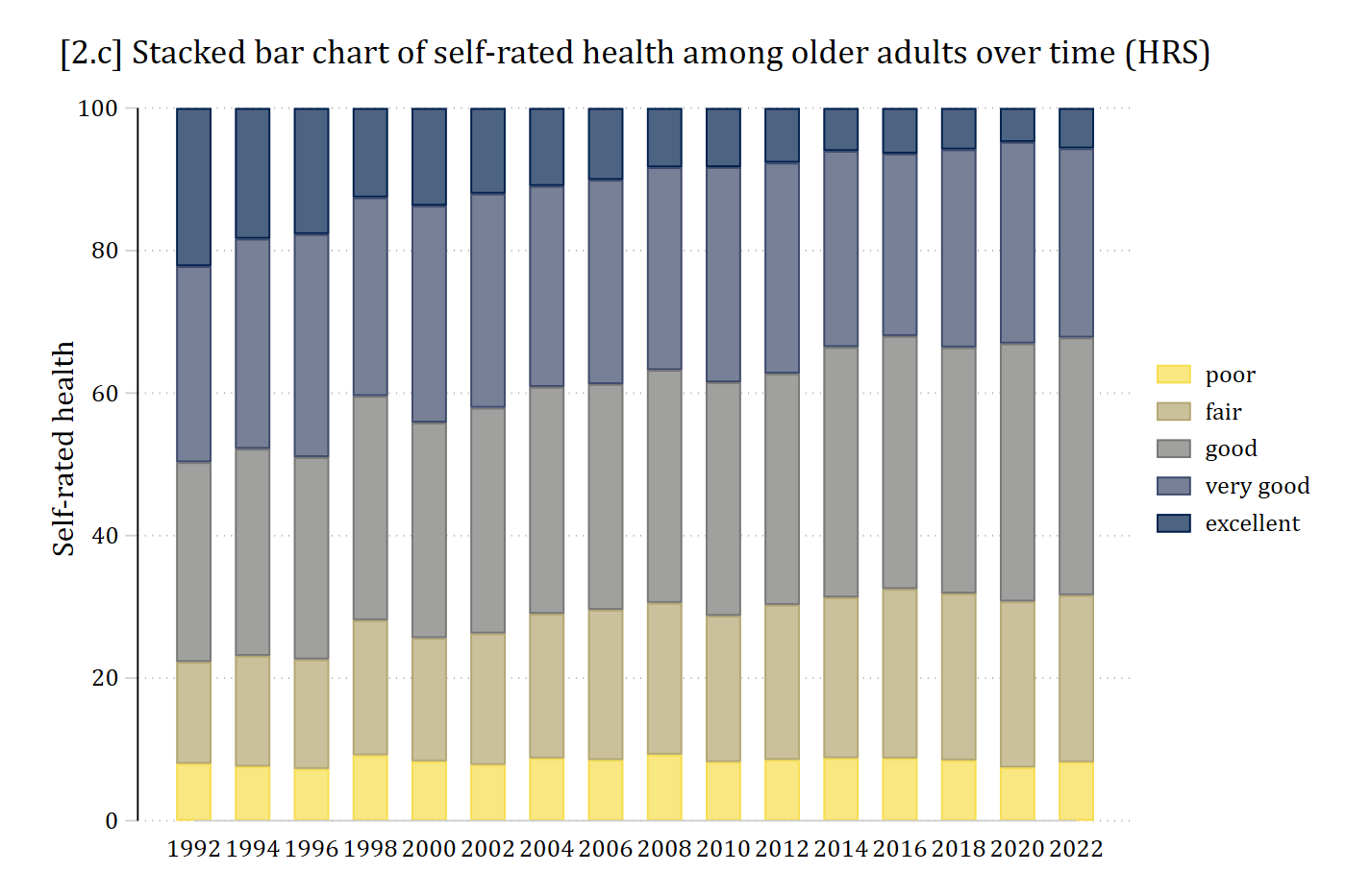
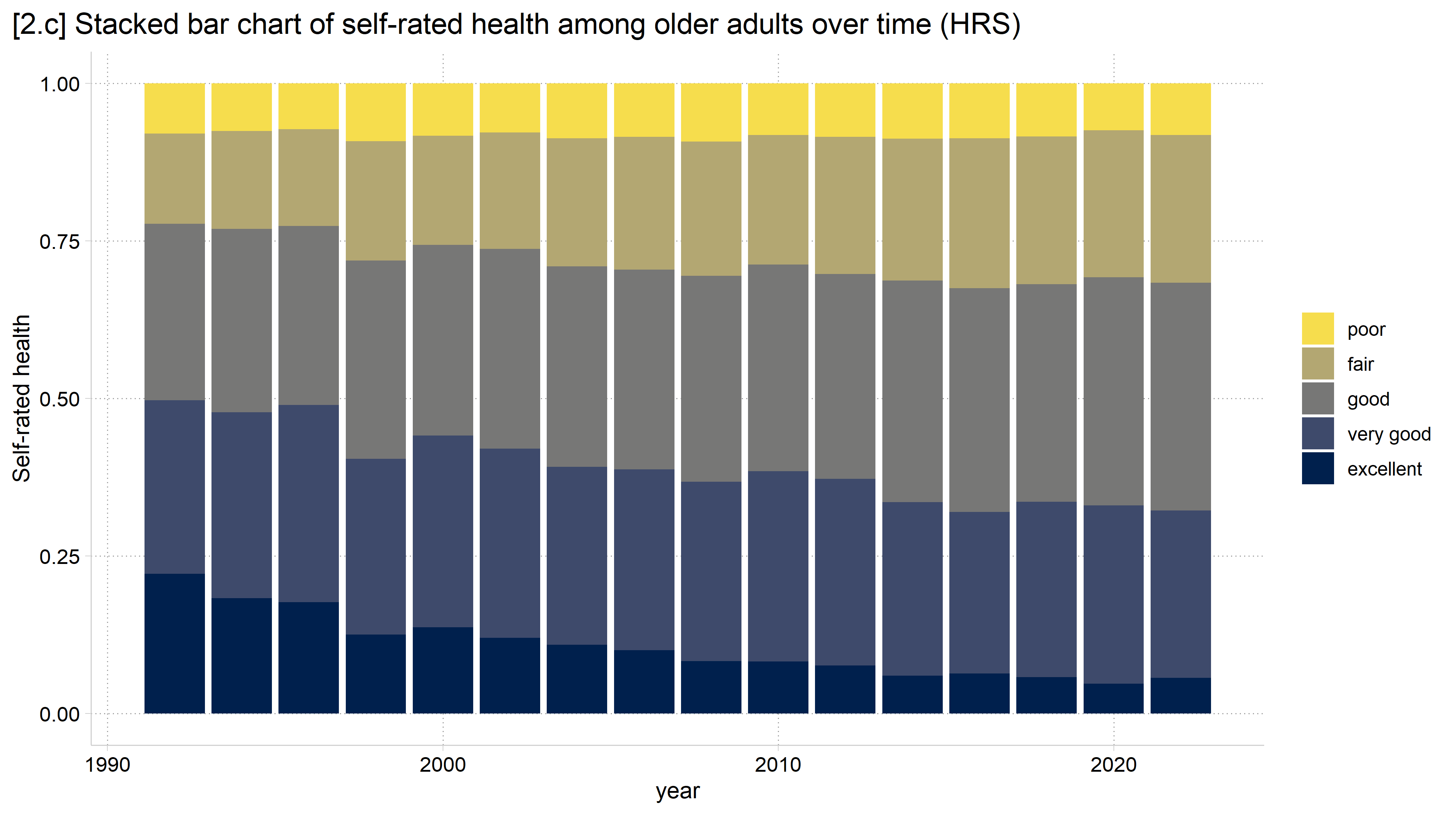
[2.c] Stacked bars of self-rated health for each HRS wave from 1992 to 2022 in the 1992 cohort: the share reporting excellent health shrinks from about 22% to about 5% over time while the shares reporting good and fair grow.

# 2.c - Stacked bar chart with 1992 cohort
ggplot(filter(hrs_filtered, !is.na(srhealth)), aes(fill = srhealth, x = year)) +
  geom_bar(position = "fill") +
  labs(title = "[2.c] Stacked bar chart of self-rated health among older adults over time (HRS)",
       y = "Self-rated health", fill = "") +
  scale_fill_viridis_d(option = "cividis", direction = -1, end = .95)

[2.c] Stacked bars of self-rated health for each HRS wave from 1992 to 2022 in the 1992 cohort: the share reporting excellent health shrinks from about 22% to about 5% over time while the shares reporting good and fair grow.

Published stacked bar chart example

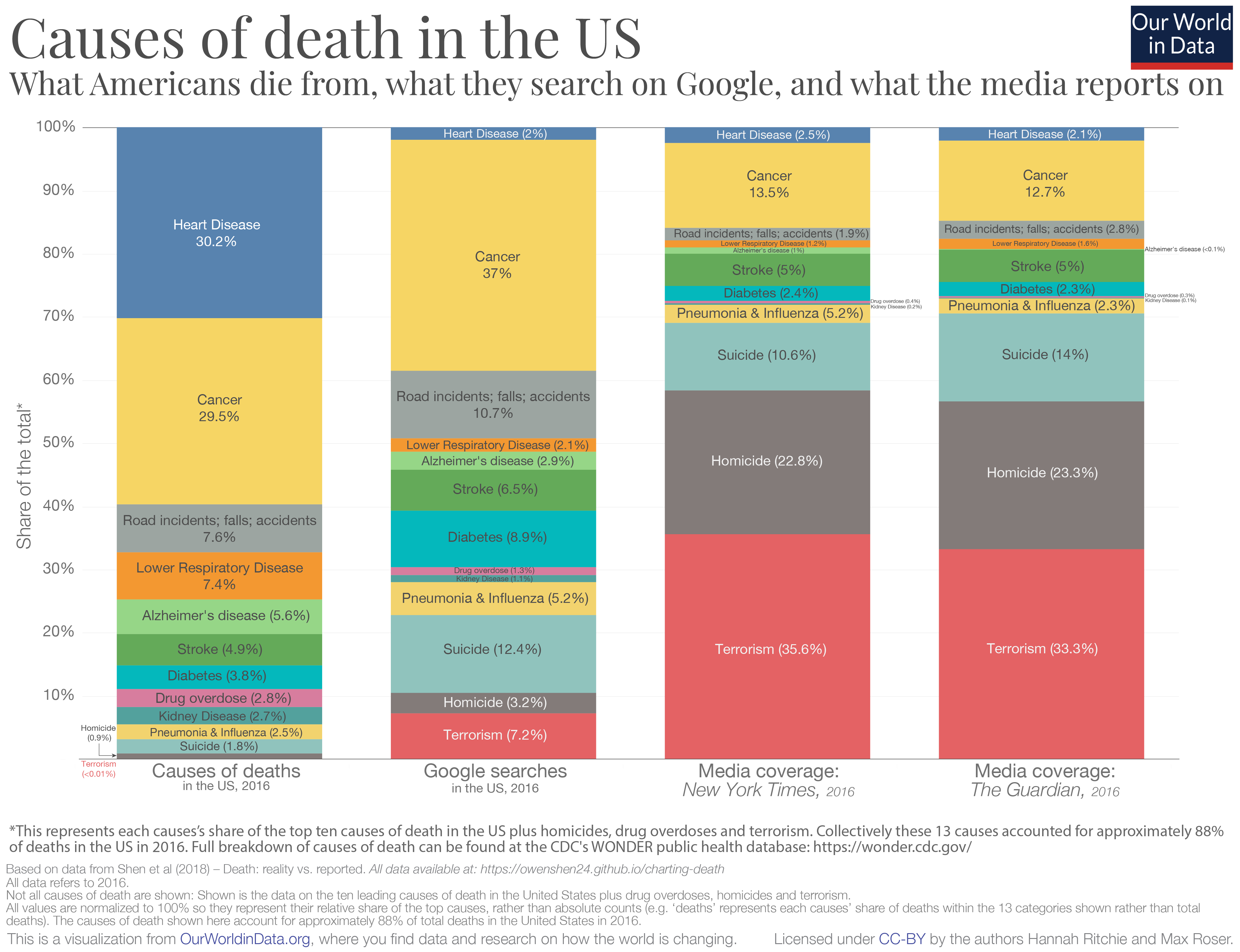
Our World in Data stacked bar chart, Causes of death in the US: what Americans die from compared with what they search on Google and what the media reports on.

Bar charts

  • The findings from the visual perception experiments pioneered by Cleveland and colleagues lead to some straightforward conclusions about effective graphics:
    • Angles are difficult to perceive accurately
      • Pie charts are not effective
    • Area is difficult to judge—especially when multiple aspects are varying at once (e.g., both length and width)
    • A common scale is necessary to compare across groups
  • Bar charts—where the width stays the same and only the length varies based on a quantitative metric—are among the most effective tools for comparing quantities

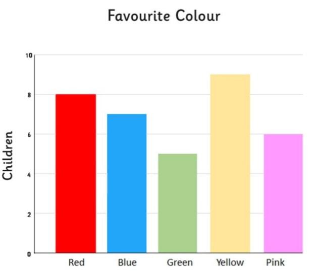
Simple bar chart of children's favourite colour: red, blue, green, yellow, and pink.

// 2.d - Bar chart for distribution of days drinking
graph bar (count), ///
    over(dayweekdrink) ///
    title("[2.d] Bar chart for days usually drink each week (older adults, HRS
)") ///
    ytitle("Count") b1title("Days usually drink each week")

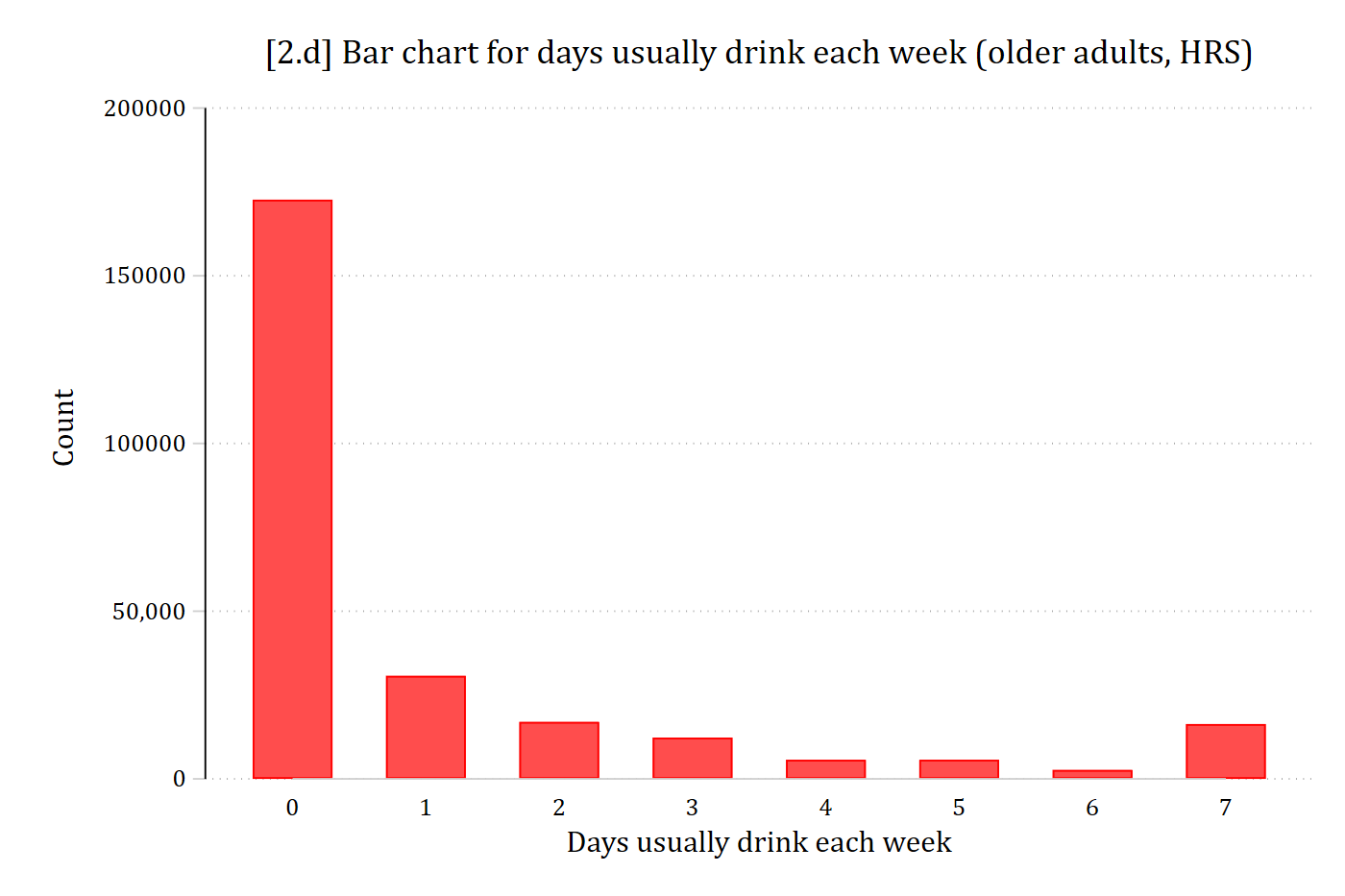
[2.d] Bar chart of the number of days older adults usually drink each week, 0 to 7: by far the tallest bar is 0 days (over 170,000 observations), followed by 1 day; the bars for 2 to 6 days are short, with a small rise at 7 days.

# 2.d - Bar chart for distribution of days drinking
ggplot(filter(hrs, !is.na(dayweekdrink)), aes(x = dayweekdrink)) +
  geom_bar() +
  labs(title = "[2.d] Bar chart for days usually drink each week (older adults, HRS)",
       x = "Days usually drink each week", y = "Count")

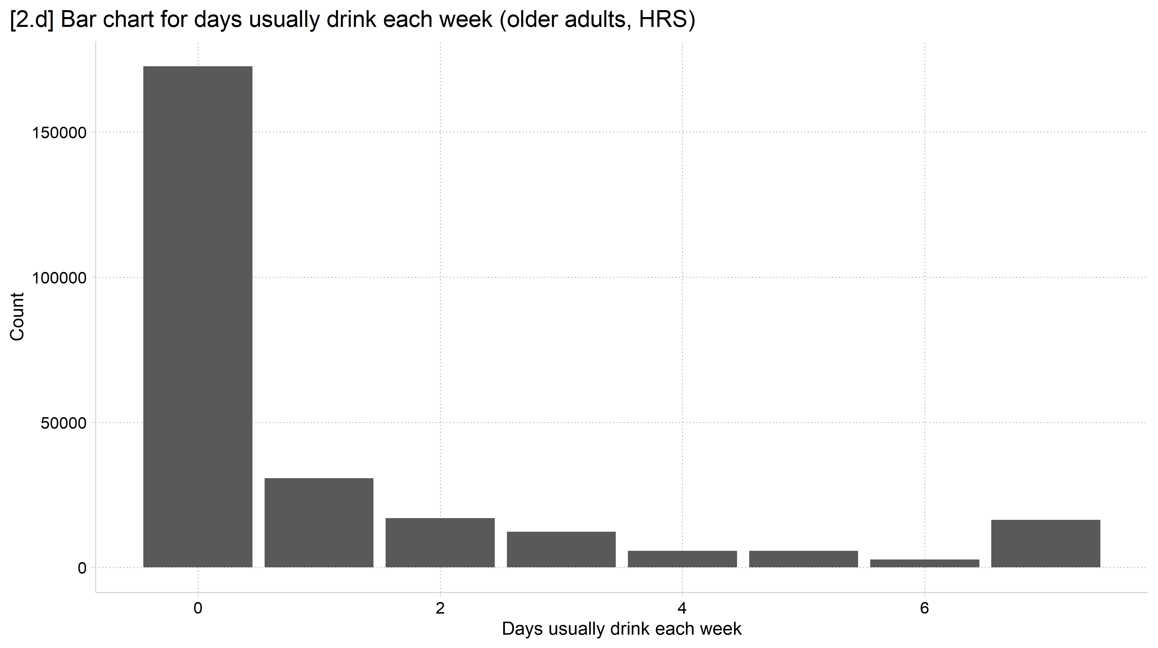
[2.d] Bar chart of the number of days older adults usually drink each week, 0 to 7: by far the tallest bar is 0 days, followed by 1 day; the bars for 2 to 6 days are short, with a small rise at 7 days.

Back to top