1.3 Linear Regression (with math)

Cartoon of a library: 'Who is putting the math books in the horror section?'

Outcome (DV) = linear combination + error

The linear regression model:

\[y_{i} = \beta_{0} + \beta x_{i} + \varepsilon_{i}\]

\[{income}_{i} = \beta_{0} + \beta_{ed\_yrs}{ed\_yrs}_{i} + \beta_{woman}{woman}_{i} + \ldots + \varepsilon_{i}\]

In matrix notation:

\[y_{i} = \mathbf{x}_{i}\boldsymbol{\beta} + \varepsilon_{i}\]

\[y_{i} = \begin{bmatrix} 1 & x_{i1} & \ldots & x_{ik} \end{bmatrix}\begin{bmatrix} \beta_{0} \\ \beta_{1} \\ \ldots \\ \beta_{k} \end{bmatrix} + \varepsilon_{i} = \beta_{0} + \beta_{1}x_{i1} + \ldots + \beta_{k}x_{ik} + \varepsilon_{i}\]

  • Note the bolded \(\mathbf{x}\) and the bolded \(\boldsymbol{\beta}\) (beta) above is notation to denote a matrix (in this case vectors [which is a matrix with only one row or column])
    • This allows for compact notation to refer to many IVs (\(\mathbf{x}\)) and many associated coefficients (\(\boldsymbol{\beta}\))
  • The x’s have subscript i’s to denote they vary across each observation in the data
    • The \(\beta\)’s do not have subscripts because there is only one for each variable

ε is unexplained variation

  • \(\varepsilon\) (epsilon) represents variation that is not explained by the IVs (\(\mathbf{x}\))
    • Often called the “error term” (or “disturbance”)
  • No health or social science model is likely to explain anywhere close to 100% of the variation in the DV so there will be some unexplained variation
    • Unexplained variation may be due to:
      • Randomness
      • Measurement error
      • Unobserved heterogeneity
        • Some sources of error were measured but not included in your model; some sources of error are unmeasurable; etc.
  • For any given observation we can calculate a prediction error—also called the residual for that observation (often denoted as \(e_{i}\) rather than \(\varepsilon_{i}\) to distinguish it from the error which is a theoretical deviation from the true value rather than the observed value)—by comparing their observed value of the DV (\(y_{i}\)) to what our model predicts (\(\widehat{y}\)) [note a “\(\widehat{hat}\)” denotes a predicted value]

\[prediction\ error = e_{i} = observed - predicted = y_{i} - {\widehat{y}}_{i}\]

Maximum likelihood and OLS estimates of β’s

  • Guess the values of the coefficients: \(\boldsymbol{\beta}^{*}\)
    • For this guess, the residuals for case i are:

\[r_{i}^{*} = y_{i} - \mathbf{x}_{i}\boldsymbol{\beta}^{*} = y_{i} - {\widehat{y}}_{i}\]

  • Compute the sum of squared residuals (total amount of error):

\[SSR = \sum_{i = 1}^{N}(y_{i} - \mathbf{x}_{i}\boldsymbol{\beta})^{2} = \sum_{i = 1}^{N}{r_{i}}^{2}\]

  • Try other values of \(\boldsymbol{\beta}^{*}\) to see if you can make SSR smaller
    • The maximum likelihood estimates of \(\boldsymbol{\beta}^{*}\) are those that make SSR the smallest
      • Much more on this later; the general intuition is OK for now
  • The ordinary least squares (OLS) estimate of \(\widehat{\boldsymbol{\beta}}\) minimizes the SSR via a mathematical solution
    • Can calculate the best \(\widehat{\boldsymbol{\beta}}\) with matrix algebra. OLS has a simple “closed-form” formula:

\[\widehat{\boldsymbol{\beta}} = (\mathbf{X}'\mathbf{X})^{-1}\mathbf{X}'\mathbf{y}\]

Properties of the OLS estimator

  • When the assumptions hold, OLS estimates are BLUE
    • Best: smallest possible sampling variance
    • For a Linear combination of the data
    • And Unbiased: on average the correct answer across samples
      • Best Linear Unbiased Estimator
  • These properties are asymptotic, but OLS can also work well for small N
    • Easy to find \(\widehat{\boldsymbol{\beta}}\) even in small samples
  • Note a common mistake: referring to the linear regression model as an OLS model. OLS is not a model; it is an estimator
    • E.g., Linear regression models can also be estimated by maximum likelihood

The Blue Man Group drumming on paint-covered drums.

Variance of the error & R2: explained variation

  • The residuals are used to estimate the variance of the error:

\[Var(\widehat{r}) = \frac{1}{N - K - 1}\sum_{i = 1}^{N}(y_{i} - {\widehat{y}}_{i})^{2} = s^{2}\]

  • R2 is the percent of the variation in y explained by the independent variables

\[R^{2} = \frac{Var(\widehat{y})}{Var(\widehat{y}) + Var(\widehat{r})} = \frac{Explained\ Variation}{Total\ Variation}\]

  • For example, if the R2 from a model regressing wages (DV) on gender (IV) is 0.05 this indicates that gender explains 5% of the variation in wages

Assumptions of the model

  1. Linearity
  2. Not perfect collinearity
  3. E(ε|x) = 0
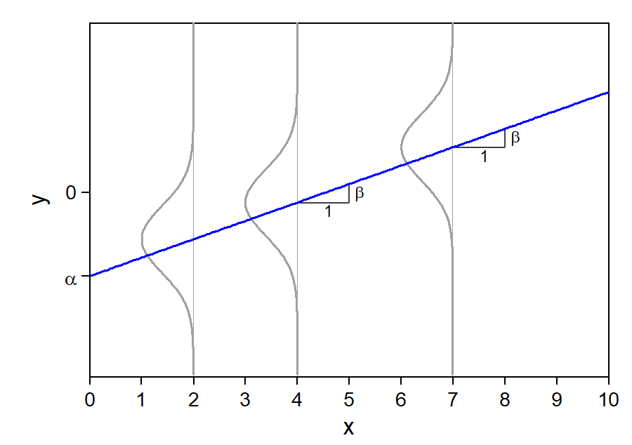
  4. Homoscedastic errors
  5. Uncorrelated errors
  6. Normally distributed errors*

A straight regression line with normal error distributions of the same spread at several values of x.

*You will commonly hear people refer to an additional—but incorrect—assumption of the model: that variables (especially the DV) must be normally distributed. This does not have to be the case, and linear regression estimates tend to be quite robust even with highly non-normal data. See Lumley et al. 2002

Linearity

  • y is linearly related to the x’s through the β’s

\[y = \beta_{0} + \beta_{1}x_{1} + \beta_{2}x_{2} + \varepsilon\]

  • A unit change in x1 has a constant effect on y
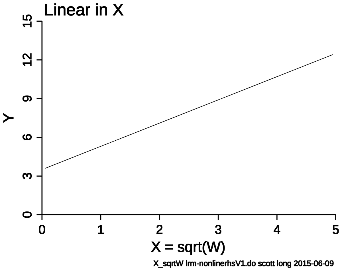
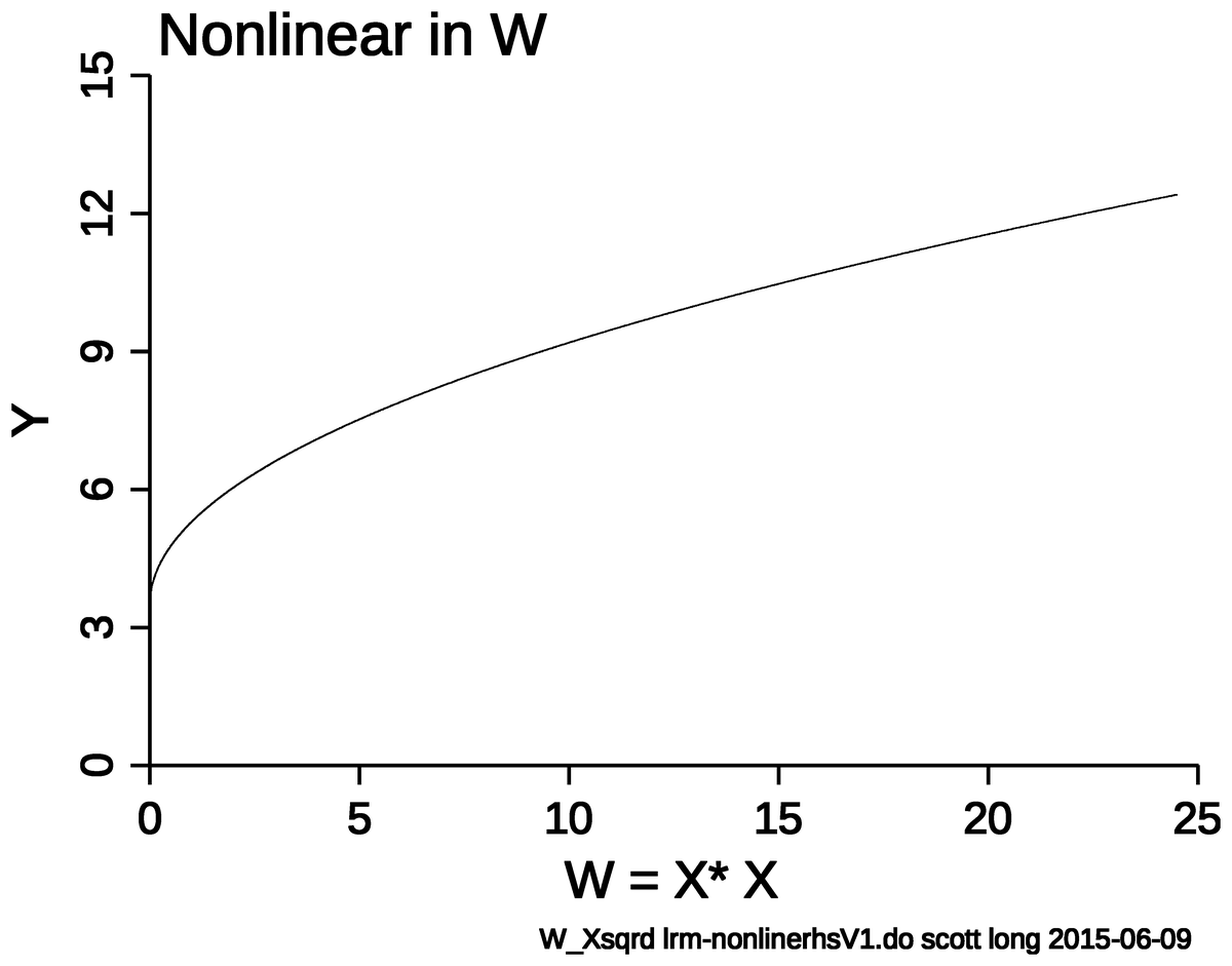
  • However, just because the model is linear does not mean the effects have to be linear. E.g., If x1 = sqrt(w1), then

\[y = \beta_{0} + \beta_{1}x_{1} + \beta_{2}x_{2} + \varepsilon = \beta_{0} + \beta_{1}\sqrt{w_{1}} + \beta_{2}x_{2} + \varepsilon\]

  • A unit change in x1 has a constant effect on y
  • A unit change in w1 does not have a constant effect on y

Y plotted against X = sqrt(W): a straight line.

Y plotted against W = X squared: a curve that rises steeply at first and then flattens.

Homoscedastic errors

  • Across all values of your IV (\(\mathbf{x}\)) you have the same variance for ε

\[Var(\varepsilon_{i}\,|\,\mathbf{x}_{i}) = \sigma^{2} \text{ for all } i \;\; (\sigma^{2} \text{ has no subscript } i)\]

  • Can you think of when this would not be the case?
    • E.g., Where for some values of your IV your model predicts well (leading to a small variance of the errors at those values) but does not predict well at other values (leading to a large variance of the errors at those values)?

Errors are uncorrelated

  • Knowing the residual for one observation does not provide any systematic information about the residual of another observation
  • Can you think of a situation where this would not be the case?
    • E.g., Where knowing how well the model predicts for one case, is associated with how well it predicts for other similar (or dissimilar) cases?

Normally distributed errors

  • The errors from your model should be approximately normally distributed for accurate significance testing
    • But, deviations from normality are common and usually do not cause major issues, especially with large datasets (Lumley et al. 2002)

Collinearity

  • We use multiple regression since the variables in \(\mathbf{x}\) are correlated (collinear)
    • The variables in \(\mathbf{x}\) cannot be perfectly collinear
      • Rarely the case unless by mistake (e.g., income in $ and income in €)
    • Collinearity is rarely an issue for overall model inference or fit; can make interpretations of specific IVs problematic
      • If two IVs are explaining the same source of variation in the DV it can be difficult to isolate the effects of each
      • Can lead to puzzling situations such as when both IVs are non-significant in the model despite overall model fit increasing markedly when both variables are added to the model
        • Possible solutions:
          • Include only one or the other variable in the model
          • Combine the variables into one measure (e.g., a scale or index)

Assessing multicollinearity

  • The most common way to assess multicollinearity is to calculate variance inflation factors (VIFs)
    • Estimate a separate linear regression for each IV x where the IV is used as the dependent variable and all other IVs are used as predictors
    • Use the R2 from that model to calculate the VIF for that IV

\[VIF = \frac{1}{1 - R^{2}}\]

  • No hard and fast rules for what VIF value is problematic
    • “The VIF has a lower bound of 1 but no upper bound. Authorities differ on how high the VIF has to be to constitute a problem. Personally, I tend to get concerned when a VIF is greater than 2.50, which corresponds to an R2 of .60 with the other variables.” (Allison 2012)

  • Read more on when you can safely ignore multicollinearity and why dropping IVs just because they are collinear is usually not a good idea
  • In Stata or R, easy to calculate VIFs
use "https://tdmize.github.io/data/data/cda_ah4", clear
(cda_ah4.dta | Add Health Wave 4 - | )
reg income edyrs i.woman i.race age health subjclass role
      Source |       SS           df       MS      Number of obs   =     4,893
-------------+----------------------------------   F(9, 4883)      =    179.60
       Model |  882023.504         9  98002.6115   Prob > F        =    0.0000
    Residual |  2664556.55     4,883  545.680228   R-squared       =    0.2487
-------------+----------------------------------   Adj R-squared   =    0.2473
       Total |  3546580.06     4,892  724.975482   Root MSE        =     23.36

-------------------------------------------------------------------------------
       income | Coefficient  Std. err.      t    P>|t|     [95% conf. interval]
--------------+----------------------------------------------------------------
        edyrs |      2.279      0.162   14.032   0.000        1.961       2.598
              |
        woman |
       Woman  |    -13.099      0.685  -19.125   0.000      -14.442     -11.756
              |
         race |
       Black  |     -4.828      0.795   -6.075   0.000       -6.386      -3.270
Native Ame..  |      3.039      3.868    0.786   0.432       -4.544      10.622
       Asian  |      4.558      1.947    2.341   0.019        0.740       8.376
              |
          age |      1.029      0.186    5.543   0.000        0.665       1.393
       health |      0.980      0.386    2.535   0.011        0.222       1.737
    subjclass |      4.097      0.216   18.927   0.000        3.673       4.522
         role |      1.777      0.229    7.751   0.000        1.327       2.226
        _cons |    -55.353      5.850   -9.462   0.000      -66.822     -43.885
-------------------------------------------------------------------------------
estat vif
    Variable |       VIF       1/VIF  
-------------+----------------------
       edyrs |      1.26    0.793448
     1.woman |      1.04    0.958210
        race |
          2  |      1.02    0.980839
          3  |      1.01    0.993158
          4  |      1.02    0.983295
         age |      1.01    0.991702
      health |      1.12    0.893390
   subjclass |      1.25    0.799726
        role |      1.07    0.932903
-------------+----------------------
    Mean VIF |      1.09
library(haven)           # import Stata data and labels
library(olsrr)           # variance inflation factors (VIFs)

ah4 <- read_dta("https://tdmize.github.io/data/data/cda_ah4.dta")

mod4 <- lm(income ~ edyrs + woman + as_factor(race) + age + health + subjclass + role,
  data = ah4)

ols_vif_tol(mod4)
                       Variables Tolerance      VIF
1                          edyrs 0.7934480 1.260322
2                          woman 0.9582097 1.043613
3           as_factor(race)Black 0.9808386 1.019536
4 as_factor(race)Native American 0.9931579 1.006889
5           as_factor(race)Asian 0.9832954 1.016988
6                            age 0.9917022 1.008367
7                         health 0.8933900 1.119332
8                      subjclass 0.7997259 1.250428
9                           role 0.9329033 1.071922
Back to top