6.6 Negative Binomial Models

\[Var(y\,|\,\mathbf{x}) = E(y\,|\,\mathbf{x}) = \exp(\mathbf{x}\boldsymbol{\beta})\]

\[Var(y\,|\,\mathbf{x}) > E(y\,|\,\mathbf{x})\]

Unobserved heterogeneity

  • In the negative binomial model, a new source of error is added

\[\mu = \exp(\beta_{0} + \beta_{1}x_{1,i} + \beta_{2}x_{2,i} + \ldots + \beta_{k}x_{k,i}) \quad \text{for the Poisson model}\]

\[\widetilde{\mu} = \exp(\beta_{0} + \beta_{1}x_{1,i} + \beta_{2}x_{2,i} + \ldots + \beta_{k}x_{k,i} + \varepsilon) \quad \text{for the negative binomial model}\]

  • ε is assumed uncorrelated with x
  • ε can be due to
    • Combined effects of excluded variables
    • Pure randomness
  • \(\widetilde{\mu}\) from NBRM and \(\mu\) from PRM are related

\[\begin{aligned} \widetilde{\mu} &= \exp(\beta_{0} + \beta_{1}x_{1} + \beta_{2}x_{2} + \beta_{3}x_{3}) \times \exp(\varepsilon) \\ &= \mu \times \exp(\varepsilon) \\ &= \mu\nu \quad \text{where } \nu \equiv \exp(\varepsilon) \end{aligned}\]

Identification & the negative binomial distribution

  • In linear regression we assume E(ε) = 0 to identify the model
    • We need a similar assumption for the negative binomial model
  • Most conveniently assume

\[E(\nu) = 1 = E[\exp(\varepsilon)]\]

  • With this assumption, Poisson and negative binomial have the same mean structure

\[E(\widetilde{\mu}) = E(\mu\nu) = \mu E(\nu) = \mu\]

Poisson distribution given x and ν

  • ν (“nu”) is unobserved, but assume we know the value of ν for each observation
    • Knowing ν, we treat it as an independent variable with βν = 1
  • The distribution of y given both x and ν is Poisson (since ν is just another x)

\[\Pr(y\,|\,\mathbf{x}, \nu) = \frac{e^{-\widetilde{\mu}}\,\widetilde{\mu}^{\,y}}{y!} = \frac{e^{-\mu\nu}(\mu\nu)^{y}}{y!}\]

  • However, ν is unobserved so we cannot compute Pr(y|x, ν)!
    • Instead, we compute Pr(y|x) by mixing across ν

Mixing distributions

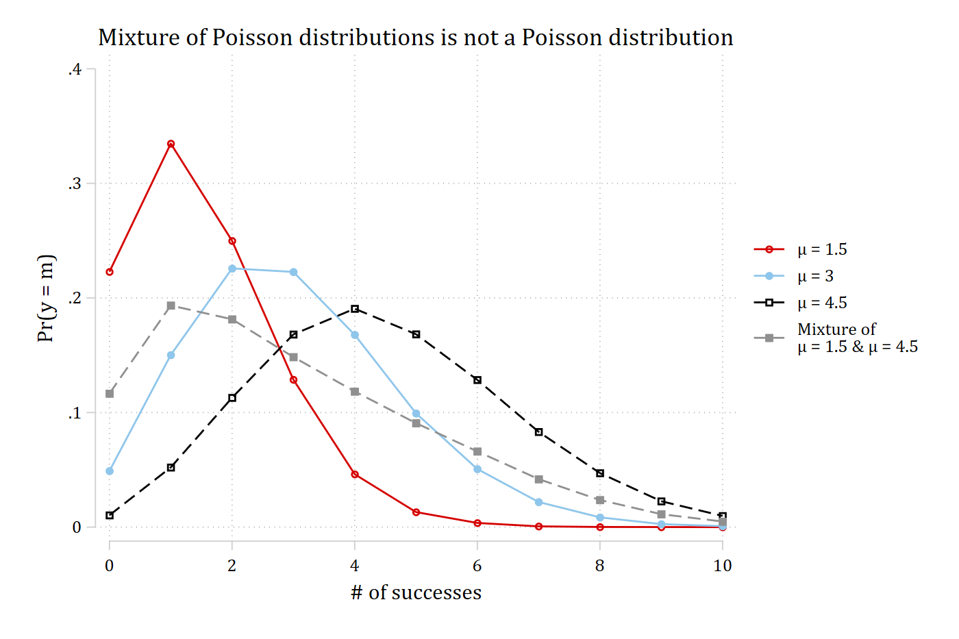
* Simulated data from 6.1 (see the code there)
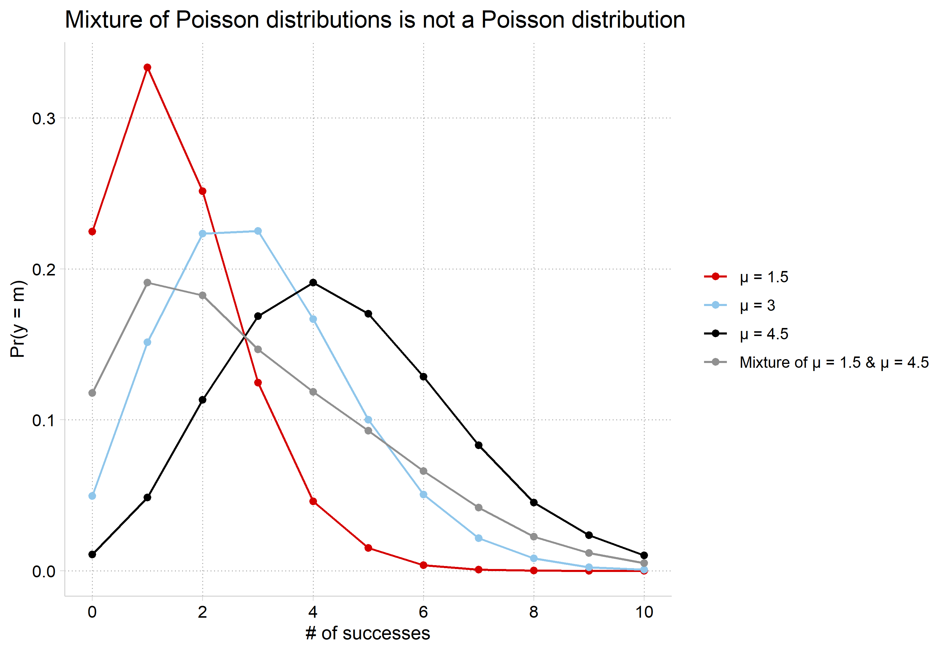
*Show that mixture of two Poissons is not Poisson
gen mixpo = (p15obeq + p45obeq) / 2
(49,989 missing values generated)
twoway ///
    connected p15obeq p15val || ///
    connected p3obeq  p3val || ///
    connected p45obeq p45val || ///
    connected mixpo p45val || ///
    , ytitle("Pr(y = m)") xtitle("# of successes") ///
    title("Mixture of Poisson distributions is not a Poisson distribution") //
/
    legend(order(1 "{&mu} = 1.5" 2 "{&mu} = 3" ///
        3 "{&mu} = 4.5" 4 "Mixture of" "{&mu} = 1.5 & {&mu} = 4.5"))

Simulated Poisson distributions with means 1.5, 3, and 4.5, and the mixture of the 1.5 and 4.5 distributions: the mixture peaks at 1 to 2 with a long right tail and does not match the Poisson distribution with mean 3, which peaks at 2 to 3.

# Simulated data from 6.1 (see the code there)

# Show that mixture of two Poissons is not Poisson
mixture <- bind_rows(
  "μ = 1.5" = pr_count(sim$y1_5, 10),
  "μ = 3" = pr_count(sim$y3, 10),
  "μ = 4.5" = pr_count(sim$y4_5, 10),
  "Mixture of μ = 1.5 & μ = 4.5" = data.frame(k = 0:10,
    pr = (pr_count(sim$y1_5, 10)$pr + pr_count(sim$y4_5, 10)$pr) / 2),
  .id = "dist") |>
  mutate(dist = factor(dist, levels = unique(dist)))

ggplot(mixture, aes(x = k, y = pr, color = dist)) +
  geom_line() + geom_point() +
  scale_x_continuous(breaks = seq(0, 10, 2)) +
  labs(title = "Mixture of Poisson distributions is not a Poisson distribution",
    x = "# of successes", y = "Pr(y = m)", color = NULL)

Simulated Poisson distributions with means 1.5, 3, and 4.5, and the mixture of the 1.5 and 4.5 distributions: the mixture peaks at 1 to 2 with a long right tail and does not match the Poisson distribution with mean 3, which peaks at 2 to 3.

Mixing distributions for the negative binomial model

  • A mixture of two Poisson distributions (e.g., μ1 = 1.5 and μ2 = 4.5) will not produce a Poisson (μ = 3) distribution
  • In the negative binomial model, the Pr(y | x) is a mixture across ν
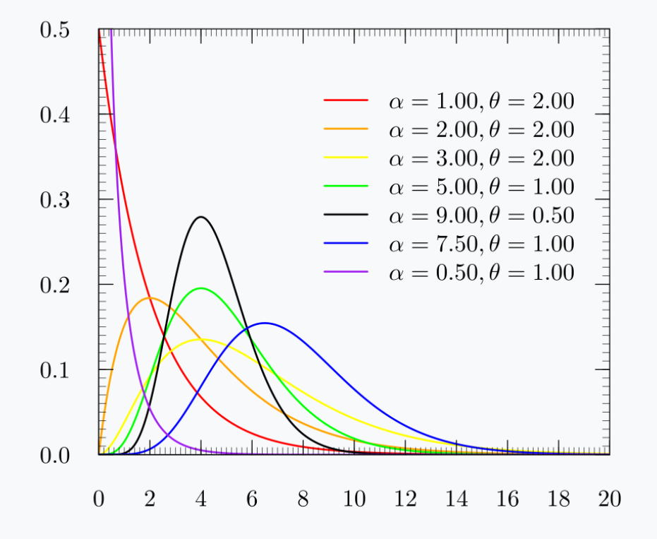
    • We assume ν has a gamma distribution with:
      • E(ν) = 1
      • Var(ν) = 1/δ ≡ α
    • The distribution varies in shape with changes in α (see below)
  • Idea is different people/groups in the data have different count processes governing their observed counts
    • Each individually is a Poisson process
      • We observe the pooled/mixed distribution in the data, which is not a Poisson
    • Details omitted due to space and time. See Long (1997) for more specifics as to how this works

Gamma distributions for seven combinations of the shape parameter alpha and scale parameter theta, from a steeply falling curve when alpha is 0.5 or 1 to hump-shaped curves that peak further right as alpha grows.

*Gamma distribution varies based on shape parameter α, which we estimate

Negative binomial distribution

  • The mixture of Poisson PDFs by gamma is a negative binomial distribution

\[\Pr(y\,|\,\mathbf{x}) = \frac{\Gamma(y + \alpha^{-1})}{y!\,\Gamma(\alpha^{-1})}\left(\frac{\alpha^{-1}}{\alpha^{-1} + \mu}\right)^{\alpha^{-1}}\left(\frac{\mu}{\alpha^{-1} + \mu}\right)^{y}\]

  • It has the same mean structure as the Poisson model. So, predicted rates are calculated in the exact same way:

\[E(y\,|\,\mathbf{x}) = \exp(\mathbf{x}\boldsymbol{\beta}) = \mu\]

  • Where the variance is larger

\[Var(y\,|\,\mathbf{x}) = \mu(1 + \alpha\mu) = \exp(\mathbf{x}\boldsymbol{\beta})(1 + \alpha\exp(\mathbf{x}\boldsymbol{\beta})) > \mu\]

  • Since μ and α are positive, the negative binomial has overdispersion

Negative binomial model example

use "https://tdmize.github.io/data/data/cda_ah4", clear
(cda_ah4.dta | Add Health Wave 4 - | )
*6.6.a
nbreg drinktime i.woman c.age i.college i.race c.income ///
    i.spouserole i.parrole, irr
Fitting Poisson model:

Iteration 0:  Log likelihood =  -11915.53  
Iteration 1:  Log likelihood = -11915.529  

Fitting constant-only model:

Iteration 0:  Log likelihood =  -9756.951  
Iteration 1:  Log likelihood =  -9665.495  
Iteration 2:  Log likelihood = -9664.4348  
Iteration 3:  Log likelihood = -9664.4348  

Fitting full model:

Iteration 0:  Log likelihood = -9484.6092  
Iteration 1:  Log likelihood = -9465.6951  
Iteration 2:  Log likelihood = -9465.4713  
Iteration 3:  Log likelihood = -9465.4713  

Negative binomial regression                            Number of obs =  4,983
                                                        LR chi2(9)    = 397.93
Dispersion: mean                                        Prob > chi2   = 0.0000
Log likelihood = -9465.4713                             Pseudo R2     = 0.0206

-------------------------------------------------------------------------------
    drinktime |        IRR   Std. err.      z    P>|z|     [95% conf. interval]
--------------+----------------------------------------------------------------
        woman |
       Woman  |      0.618      0.026  -11.631   0.000        0.569       0.670
          age |      0.949      0.011   -4.713   0.000        0.929       0.970
              |
      college |
College De..  |      0.756      0.035   -6.112   0.000        0.691       0.827
              |
         race |
       Black  |      0.718      0.034   -6.953   0.000        0.653       0.788
Native Ame..  |      1.332      0.282    1.353   0.176        0.879       2.019
       Asian  |      0.897      0.101   -0.964   0.335        0.718       1.119
              |
       income |      1.003      0.001    4.040   0.000        1.002       1.005
              |
   spouserole |
     Married  |      0.884      0.038   -2.887   0.004        0.812       0.961
              |
      parrole |
      Parent  |      0.777      0.035   -5.658   0.000        0.712       0.848
        _cons |     14.481      4.518    8.567   0.000        7.857      26.691
--------------+----------------------------------------------------------------
     /lnalpha |      0.284      0.034                         0.217       0.352
--------------+----------------------------------------------------------------
        alpha |      1.329      0.046                         1.243       1.421
-------------------------------------------------------------------------------
Note: Estimates are transformed only in the first equation to incidence-rate
      ratios.
Note: _cons estimates baseline incidence rate.
LR test of alpha=0: chibar2(01) = 4900.12              Prob >= chibar2 = 0.000
est store nbmod
est table nbmod, ///
    title("[6.6.a] Negative binomial regression for # of drinks in a sitting")
 ///
    b(%5.3f) star(.05 .01 .001) eform
[6.6.a] Negative binomial regression for # of drinks in a sitting

---------------------------
    Variable |   nbmod     
-------------+-------------
drinktime    |
       woman |
      Woman  |   0.618***  
         age |   0.949***  
             |
     college |
College D..  |   0.756***  
             |
        race |
      Black  |   0.718***  
Native Am..  |   1.332     
      Asian  |   0.897     
             |
      income |   1.003***  
             |
  spouserole |
    Married  |   0.884**   
             |
     parrole |
     Parent  |   0.777***  
       _cons |  14.481***  
-------------+-------------
    /lnalpha |   1.329***  
---------------------------
Legend: * p<.05; ** p<.01; *** p<.001
library(haven)           # import Stata data and labels
library(MASS)            # negative binomial: glm.nb()
library(pscl)            # odTest()
library(modelsummary)    # regression tables
library(marginaleffects) # predictions and marginal effects

ah4 <- read_dta("https://tdmize.github.io/data/data/cda_ah4.dta")

# Keep model variables; drop any missing data
ah4 <- ah4[c("drinktime", "woman", "age", "college", "race", "income", "spouserole",
  "parrole")]
ah4 <- ah4[complete.cases(ah4), ]
ah4 <- ah4 |>
  mutate(across(c(woman, college, race, spouserole, parrole), as_factor))

# 6.6.a
nbmod <- glm.nb(drinktime ~ woman + age + college + race + income + spouserole + parrole,
  data = ah4)
summary(nbmod)

Call:
glm.nb(formula = drinktime ~ woman + age + college + race + income + 
    spouserole + parrole, data = ah4, init.theta = 0.7523991106, 
    link = log)

Coefficients:
                        Estimate Std. Error z value Pr(>|z|)    
(Intercept)            2.6728422  0.3081054   8.675  < 2e-16 ***
womanWoman            -0.4818746  0.0413848 -11.644  < 2e-16 ***
age                   -0.0521753  0.0108797  -4.796 1.62e-06 ***
collegeCollege Degree -0.2802164  0.0453204  -6.183 6.29e-10 ***
raceBlack             -0.3318798  0.0477257  -6.954 3.55e-12 ***
raceNative American    0.2868363  0.2122497   1.351  0.17656    
raceAsian             -0.1089853  0.1131841  -0.963  0.33560    
income                 0.0032692  0.0007688   4.252 2.12e-05 ***
spouseroleMarried     -0.1237700  0.0434117  -2.851  0.00436 ** 
parroleParent         -0.2523594  0.0448766  -5.623 1.87e-08 ***
---
Signif. codes:  0 '***' 0.001 '**' 0.01 '*' 0.05 '.' 0.1 ' ' 1

(Dispersion parameter for Negative Binomial(0.7524) family taken to be 1)

    Null deviance: 5685.0  on 4982  degrees of freedom
Residual deviance: 5261.8  on 4973  degrees of freedom
AIC: 18953

Number of Fisher Scoring iterations: 1

              Theta:  0.7524 
          Std. Err.:  0.0258 

 2 x log-likelihood:  -18930.9430 
# Exponentiated coefficients
exp(coef(nbmod))
          (Intercept)            womanWoman                   age collegeCollege Degree 
           14.4810684             0.6176245             0.9491625             0.7556202 
            raceBlack   raceNative American             raceAsian                income 
            0.7175736             1.3322062             0.8967436             1.0032746 
    spouseroleMarried         parroleParent 
            0.8835831             0.7769654 

In Stata, use the nbreg command

In R, use the glm.nb function in the MASS package

As with Poisson, we usually exponentiate the coefficients to interpret them as factor changes on the rate:

  • Women’s rates of drinking are lower than men’s by a factor of .62
  • Each additional year of age is associated with a .95 lower rate of drinking
  • Etc.

Comparing Poisson and negative binomial

*6.6.b re-estimate Poisson for comparison to nbreg
qui poisson drinktime i.woman c.age i.college i.race c.income ///
    i.spouserole i.parrole, nolog
est store pmod
est table pmod nbmod, stats(N r2_p bic) eform b(%9.3f) t(%6.3f) vsquish ///
    title("[6.6.b] Comparison of Poisson and Neg. Binomial Estimates")
[6.6.b] Comparison of Poisson and Neg. Binomial Estimates

--------------------------------------
    Variable |   pmod        nbmod    
-------------+------------------------
drinktime    |
       woman |
      Woman  |     0.609       0.618  
             |   -23.208     -11.631  
         age |     0.951       0.949  
             |    -9.265      -4.713  
     college |
College D..  |     0.777       0.756  
             |   -10.869      -6.112  
        race |
      Black  |     0.693       0.718  
             |   -14.069      -6.953  
Native Am..  |     1.330       1.332  
             |     3.085       1.353  
      Asian  |     0.876       0.897  
             |    -2.282      -0.964  
      income |     1.003       1.003  
             |     7.931       4.040  
  spouserole |
    Married  |     0.877       0.884  
             |    -6.065      -2.887  
     parrole |
     Parent  |     0.798       0.777  
             |    -9.697      -5.658  
       _cons |    14.040      14.481  
             |    17.153       8.567  
-------------+------------------------
    /lnalpha |                 1.329  
             |                 8.303  
-------------+------------------------
Statistics   |                        
           N |      4983        4983  
        r2_p |     0.063       0.021  
         bic | 23916.196   19024.594  
--------------------------------------
                           Legend: b/t
# 6.6.b re-estimate Poisson for comparison to the negative binomial
pmod <- glm(drinktime ~ woman + age + college + race + income + spouserole + parrole,
  family = "poisson", data = ah4)

modelsummary(list("Poisson" = pmod, "Neg. Binomial" = nbmod), exponentiate = TRUE,
  statistic = "statistic", gof_map = c("nobs", "bic"),
  title = "[6.6.b] Comparison of Poisson and Neg. Binomial Estimates")
[6.6.b] Comparison of Poisson and Neg. Binomial Estimates
Poisson Neg. Binomial
(Intercept) 14.040 14.481
(17.153) (8.675)
womanWoman 0.609 0.618
(-23.208) (-11.644)
age 0.951 0.949
(-9.265) (-4.796)
collegeCollege Degree 0.777 0.756
(-10.869) (-6.183)
raceBlack 0.693 0.718
(-14.069) (-6.954)
raceNative American 1.330 1.332
(3.085) (1.351)
raceAsian 0.876 0.897
(-2.282) (-0.963)
income 1.003 1.003
(7.931) (4.252)
spouseroleMarried 0.877 0.884
(-6.065) (-2.851)
parroleParent 0.798 0.777
(-9.697) (-5.623)
Num.Obs. 4983 4983
BIC 23916.2 19024.6

Estimates of the factor change on the rate (the exponentiated coefficients) are very similar; test statistics (z) are quite different; fit statistics clearly favor negative binomial (more on this soon)

Testing for overdispersion

  • With overdispersion, Poisson estimates are inefficient with standard errors that are biased
    • You will almost always find evidence of overdispersion in real data examples
  • We test H0: α = 0 since when α = 0 the negative binomial is equivalent to Poisson
  • A likelihood ratio test of H0: α = 0 is

\[G^{2} = 2(\ln L_{NBRM} - \ln L_{PRM})\]

  • Stata reports this test automatically as the last line in the nbreg output
    • odTest in R provides the test

From the last line of the nbreg output above:

LR test of alpha=0: chibar2(01) = 4900.12              Prob >= chibar2 = 0.000
odTest(nbmod)
Likelihood ratio test of H0: Poisson, as restricted NB model:
n.b., the distribution of the test-statistic under H0 is non-standard
e.g., see help(odTest) for details/references

Critical value of test statistic at the alpha= 0.05 level: 2.7055 
Chi-Square Test Statistic =  4900.1155 p-value = < 2.2e-16 
  • In this example, there is strong evidence of overdispersion

There is evidence of overdispersion, suggesting the Poisson model is not appropriate and instead favoring a negative binomial model.

Interpretation in the negative binomial model

  • Interpretation based on rates is identical to Poisson
  • The same methods for predicted probabilities can be used although the formula for calculating predicted probabilities is much less user-friendly:

\[\Pr(y\,|\,\mathbf{x}) = \frac{\Gamma(y + \widehat{\alpha}^{-1})}{y!\,\Gamma(\widehat{\alpha}^{-1})}\left(\frac{\widehat{\alpha}^{-1}}{\widehat{\alpha}^{-1} + \widehat{\mu}}\right)^{\widehat{\alpha}^{-1}}\left(\frac{\widehat{\mu}}{\widehat{\alpha}^{-1} + \widehat{\mu}}\right)^{y}\]

  • Poisson and negative binomial tend to differ more in predictions for specific counts (especially zeroes) than in predictions for the rate
*6.6.c - Compare predictions on rate from Poisson and nbreg
est restore nbmod
(results nbmod are active now)
qui margins, at(income=(0(5)200)) saving(nbpred, replace)
est restore pmod
(results pmod are active now)
qui margins, at(income=(0(5)200)) saving(ppred, replace)
combomarginsplot ppred nbpred, noci file1opts(msym(i)) ///
    file2opts(msym(i)) xlab(0(25)200) ylab(0(1)4) ///
    legend(order(1 "Poisson" 2 "Neg. Binomial")) ///
    ytitle("Number of Drinks") xtitle("Income in $1,000s") ///
    title("[6.6.c] Comparison of Predictions for Income - Poisson vs Negative 
Binomial", size(medium))
  Variables that uniquely identify margins: income _filenumber

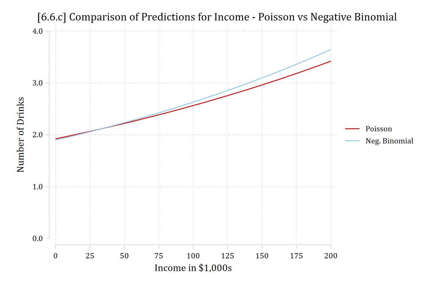
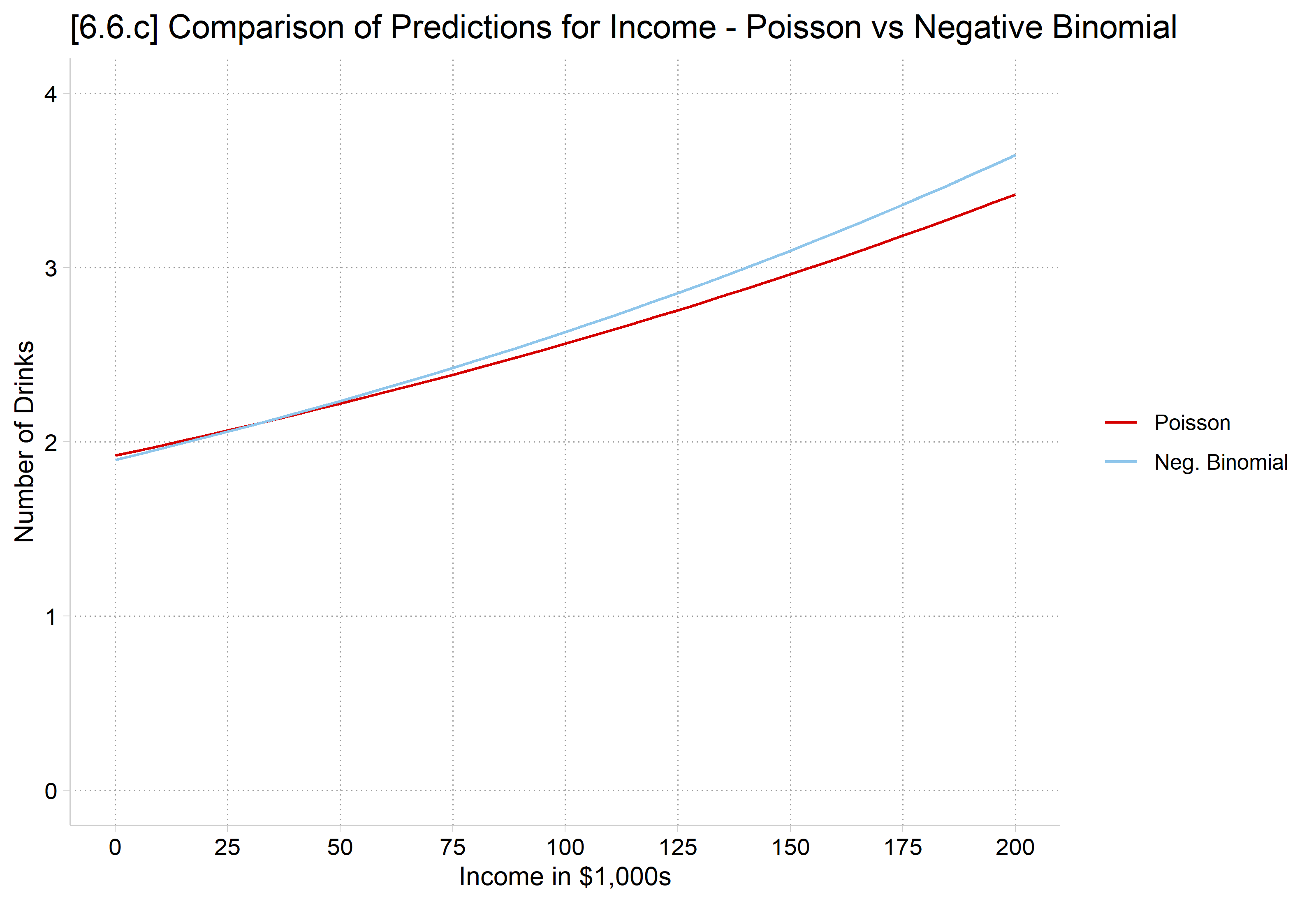
[6.6.c] Predicted number of drinks by income from the Poisson and negative binomial models: both rise from about 1.9 at no income, to about 3.4 (Poisson) and 3.6 (negative binomial) at $200,000, so the two models' predicted rates are very close.

# 6.6.c - Compare predictions on rate from Poisson and negative binomial
pr_income <- bind_rows(
  "Poisson" = avg_predictions(pmod, by = "income",
    newdata = datagrid(income = seq(0, 200, 5), grid_type = "counterfactual")),
  "Neg. Binomial" = avg_predictions(nbmod, by = "income",
    newdata = datagrid(income = seq(0, 200, 5), grid_type = "counterfactual")),
  .id = "model") |>
  mutate(model = factor(model, levels = c("Poisson", "Neg. Binomial")))

ggplot(pr_income, aes(x = income, y = estimate, color = model)) +
  geom_line() +
  scale_x_continuous(breaks = seq(0, 200, 25)) +
  scale_y_continuous(breaks = 0:4, limits = c(0, 4)) +
  labs(title = "[6.6.c] Comparison of Predictions for Income - Poisson vs Negative Binomial",
    x = "Income in $1,000s", y = "Number of Drinks", color = NULL)

[6.6.c] Predicted number of drinks by income from the Poisson and negative binomial models: both rise from about 1.9 at no income, to about 3.4 (Poisson) and 3.6 (negative binomial) at $200,000, so the two models' predicted rates are very close.

Predictions for the rate (# of drinks) are very close

*6.6.d - Compare predictions on Pr(y=0)
est restore nbmod
(results nbmod are active now)
qui margins, at(income=(0(5)200)) predict(pr(0)) saving(nbpred, replace)
est restore pmod
(results pmod are active now)
qui margins, at(income=(0(5)200)) predict(pr(0)) saving(ppred, replace)
combomarginsplot ppred nbpred, file1opts(msym(i)) ///
    file2opts(msym(i)) xlab(0(25)200) ylab(0(.1).5) ///
    recastci(rline) ciopts(lpat(dash) col(gs12)) ///
    legend(order(3 "Poisson" 4 "Neg. Binomial")) ///
    ytitle("Pr(Drinks = 0)") xtitle("Income in $1,000s") ///
    title("[6.6.d] Comparison of Pr(Zero Drinks) for Income - Poisson vs Negat
ive Binomial", size(medium))
  Variables that uniquely identify margins: income _filenumber

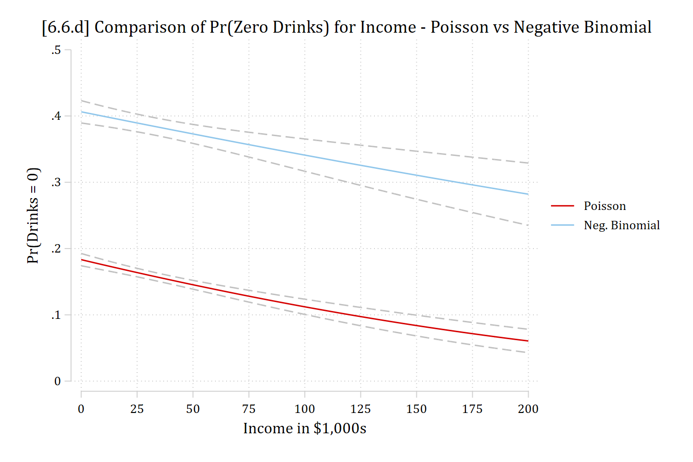
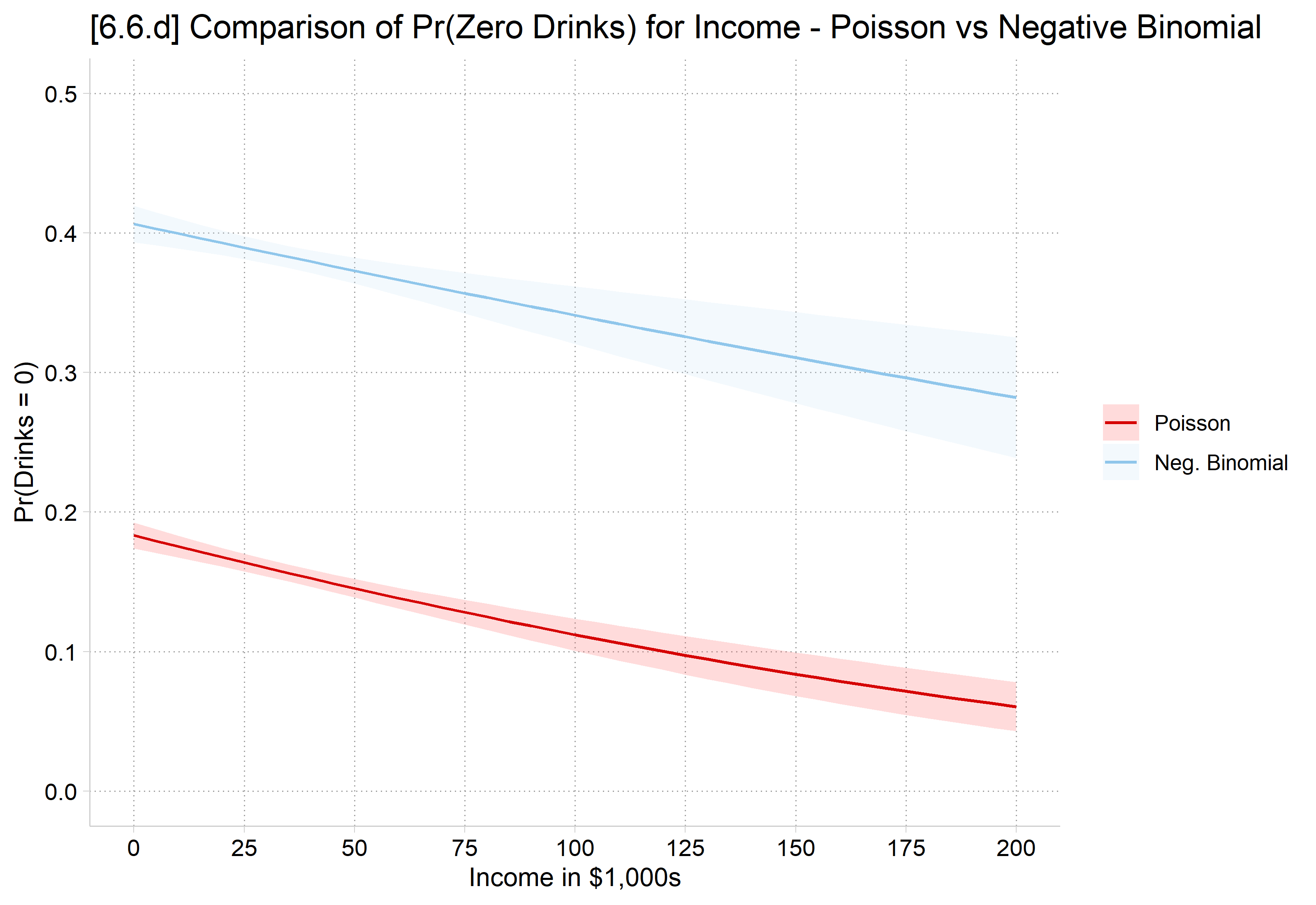
[6.6.d] Probability of zero drinks by income from the Poisson and negative binomial models, with confidence intervals: the negative binomial predicts about 0.40 at no income falling to 0.28 at $200,000, while the Poisson predicts much lower probabilities, about 0.18 falling to 0.06.

# 6.6.d - Compare predictions on Pr(y=0)
pr0_income <- bind_rows(
  "Poisson" = predictions(pmod, type = "response",
    newdata = datagrid(income = seq(0, 200, 5), grid_type = "counterfactual"),
    hypothesis = ~ I(mean(dpois(0, x))) | income),
  "Neg. Binomial" = predictions(nbmod, type = "response",
    newdata = datagrid(income = seq(0, 200, 5), grid_type = "counterfactual"),
    hypothesis = ~ I(mean(dnbinom(0, size = nbmod$theta, mu = x))) | income),
  .id = "model") |>
  mutate(model = factor(model, levels = c("Poisson", "Neg. Binomial")))

ggplot(pr0_income, aes(x = income, y = estimate, ymin = conf.low, ymax = conf.high,
    color = model, fill = model)) +
  geom_ribbon(alpha = .2, color = NA) + geom_line() +
  scale_x_continuous(breaks = seq(0, 200, 25)) +
  scale_y_continuous(breaks = seq(0, .5, .1), limits = c(0, .5)) +
  labs(title = "[6.6.d] Comparison of Pr(Zero Drinks) for Income - Poisson vs Negative Binomial",
    x = "Income in $1,000s", y = "Pr(Drinks = 0)", color = NULL, fill = NULL)

[6.6.d] Probability of zero drinks by income from the Poisson and negative binomial models, with confidence intervals: the negative binomial predicts about 0.40 at no income falling to 0.28 at $200,000, while the Poisson predicts much lower probabilities, about 0.18 falling to 0.06.

Probability y = 0 (person generally consumes zero drinks) differ considerably

Predictions and marginal effects in negative binomial models

  • Interpretation of predictions and marginal effects is identical across negative binomial and Poisson models
  • Stata and R tools for predictions and marginal effects are identical for negative binomial and Poisson
*6.6.f - Predicted # of drinks across range of age, for men and women
est restore nbmod
(results nbmod are active now)
qui margins woman, at(age=(21(1)35))
marginsplot, recastci(rline) ciopts(lpat(dash) col(gs12)) ylab(0(1)5) xlab(21(
2)35) ///
    ytitle("# of drinks") xtitle("Age in Years") ///
    title("[6.6.f] Predicted Number of Alcoholic Drinks in a Typical Sitting",
 size(medium))
Variables that uniquely identify margins: age woman

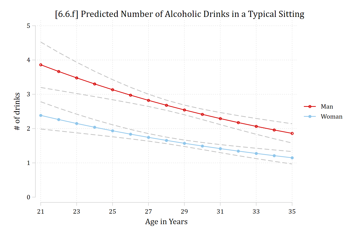
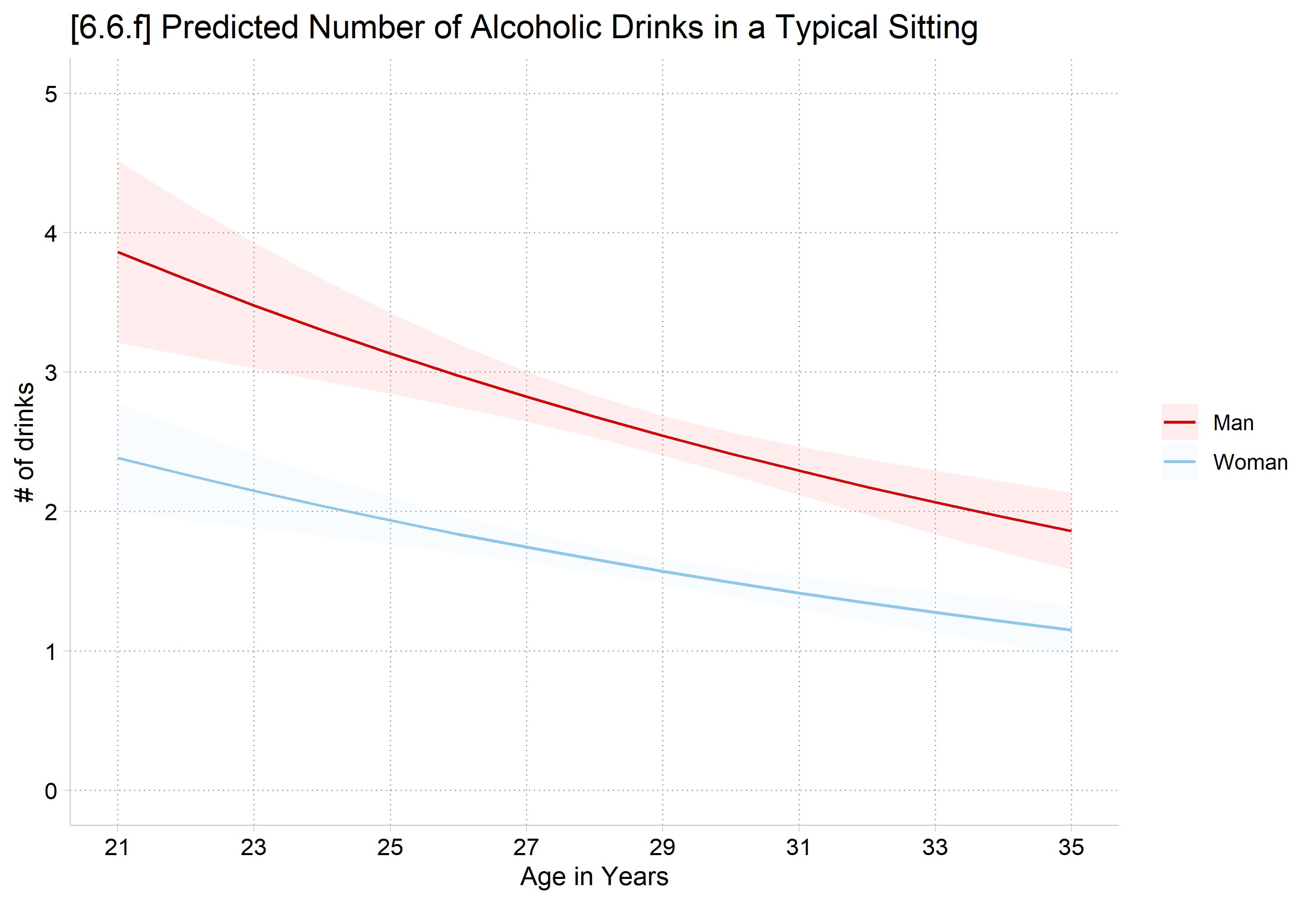
[6.6.f] Negative binomial predicted number of drinks by age, with confidence intervals: men's predictions fall from about 3.9 at age 21 to 1.9 at 35, and women's from about 2.4 to 1.2.

In R, for probabilities, specify the negative binomial formula instead of Poisson; see the examples below

# 6.6.f - Predicted # of drinks across range of age, for men and women
plot_predictions(nbmod, by = c("age", "woman"),
  newdata = datagrid(age = 21:35, woman = unique, grid_type = "counterfactual")) +
  scale_x_continuous(breaks = seq(21, 35, 2)) +
  scale_y_continuous(breaks = 0:5, limits = c(0, 5)) +
  labs(title = "[6.6.f] Predicted Number of Alcoholic Drinks in a Typical Sitting",
    x = "Age in Years", y = "# of drinks", color = NULL, fill = NULL)

[6.6.f] Negative binomial predicted number of drinks by age, with confidence intervals: men's predictions fall from about 3.9 at age 21 to 1.9 at 35, and women's from about 2.4 to 1.2.

Marginal effects on the rate

mecompare woman age, model(nbmod) amount(trimrange)
Predicting: Predicted number of events
Marginal effects (N_nbmod=4983)

                                 |  ME #   Estimate         SE      P>|z|
---------------------------------+---------------------------------------
woman                            |                                       
                 Woman - Man     |                                       
                           nbmod |     1     -1.008      0.090      0.000
---------------------------------+---------------------------------------
age(5-95%)                       |                                       
                           nbmod |     2     -0.551      0.117      0.000
avg_comparisons(nbmod, variables = list(woman = "reference", age = c(26, 31)))

  Term    Contrast Estimate Std. Error      z Pr(>|z|)    S  2.5 % 97.5 %
 age   31 - 26       -0.551     0.1154  -4.77   <0.001 19.1 -0.777 -0.325
 woman Woman - Man   -1.008     0.0897 -11.24   <0.001 95.0 -1.184 -0.832

Type: response

On average, women report drinking 1.01 fewer drinks than men

The oldest adults in this sample are predicted to drink about 0.55 fewer drinks per sitting than the youngest adults

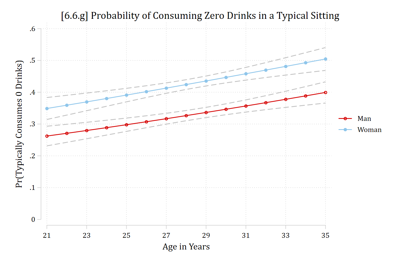
*6.6.g - Pr(y=0) across range of age, for men and women
est restore nbmod
(results nbmod are active now)
qui margins woman, at(age=(21(1)35)) predict(pr(0))
marginsplot, recastci(rline) ciopts(lpat(dash) col(gs12)) ylab(0(.1).6) xlab(2
1(2)35) ///
    ytitle("Pr(Typically Consumes 0 Drinks)") xtitle("Age in Years") ///
    title("[6.6.g] Probability of Consuming Zero Drinks in a Typical Sitting",
 size(medium))
Variables that uniquely identify margins: age woman

[6.6.g] Negative binomial probability of typically consuming zero drinks by age, with confidence intervals: it rises from about 0.26 at age 21 to 0.40 at 35 for men and from about 0.35 to 0.50 for women.

# 6.6.g - Pr(y=0) across range of age, for men and women
pr0_nb <- predictions(nbmod, type = "response",
  newdata = datagrid(age = 21:35, woman = unique, grid_type = "counterfactual"),
  hypothesis = ~ I(mean(dnbinom(0, size = nbmod$theta, mu = x))) | age + woman)

ggplot(pr0_nb, aes(age, estimate, ymin = conf.low, ymax = conf.high, color = woman, fill = woman)) +
  geom_ribbon(alpha = .2, color = NA) + geom_line() +
  scale_x_continuous(breaks = seq(21, 35, 2)) +
  scale_y_continuous(breaks = seq(0, .6, .1), limits = c(0, .6)) +
  labs(title = "[6.6.g] Probability of Consuming Zero Drinks in a Typical Sitting",
    x = "Age in Years", y = "Pr(Typically Consumes 0 Drinks)", color = NULL, fill = NULL)

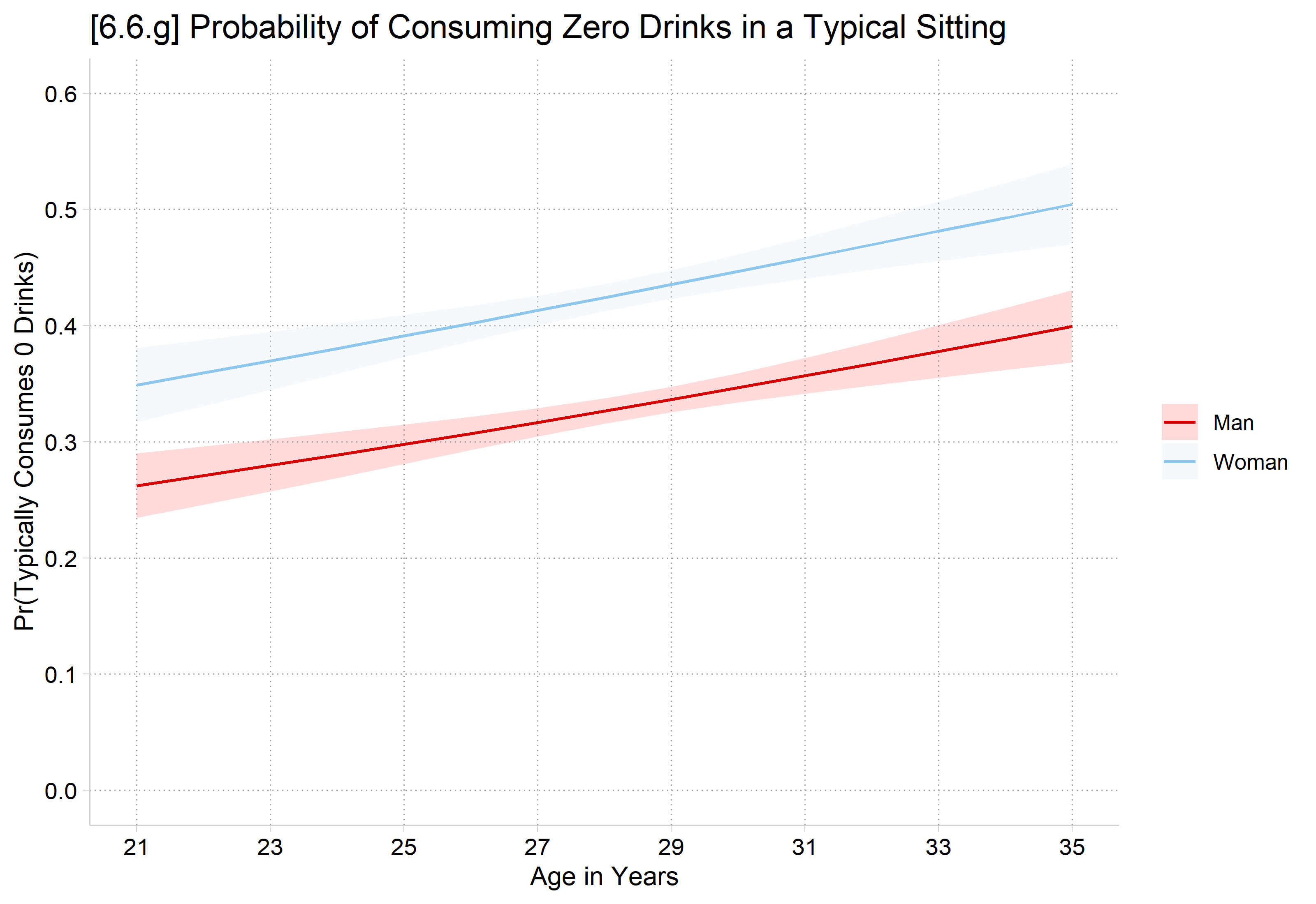
[6.6.g] Negative binomial probability of typically consuming zero drinks by age, with confidence intervals: it rises from about 0.26 at age 21 to 0.40 at 35 for men and from about 0.35 to 0.50 for women.

Marginal effects on the probability of count #

mecompare woman age, model(nbmod) amount(trimrange) predict(pr(0))
Predicting: Pr(drinktime=0)
Marginal effects (N_nbmod=4983)

                                 |  ME #   Estimate         SE      P>|z|
---------------------------------+---------------------------------------
woman                            |                                       
                 Woman - Man     |                                       
                           nbmod |     1      0.098      0.008      0.000
---------------------------------+---------------------------------------
age(5-95%)                       |                                       
                           nbmod |     2      0.053      0.011      0.000

In R, for Pr(y = #) with negative binomial models, use dnbinom(). Negative binomial probabilities depend on both the predicted count and the overdispersion parameter, so supply both: dnbinom(#, size = nbmod$theta, mu = x).

avg_comparisons(nbmod, variables = list(woman = "reference", age = c(26, 31)),
  comparison = function(hi, lo)
    dnbinom(0, size = nbmod$theta, mu = hi) - dnbinom(0, size = nbmod$theta, mu = lo))

  Term   Contrast Estimate Std. Error     z Pr(>|z|)     S  2.5 % 97.5 %
 age   custom       0.0529    0.01104  4.79   <0.001  19.2 0.0313 0.0746
 woman Woman, Man   0.0980    0.00841 11.65   <0.001 101.9 0.0816 0.1145

Type: response

Women’s average probability of having zero drinks is about 10 percentage points higher than men’s.

Across the trimmed range of age, the probability of having zero drinks increases by about .05.
*6.5.b
est restore pmod
(results pmod are active now)
qui mgen, pr(0/18) meanpred stub(pmod) replace
est restore nbmod
(results nbmod are active now)
qui mgen, pr(0/18) meanpred stub(nb) replace
twoway connected pmodobeq pmodpreq nbpreq pmodval, ylab(0(.1).45) xlab(0(2)18)
 ///
    ytitle("Pr(y = k)") xtitle("Number of Drinks in Typical Sitting") ///
    title("[6.5.b] Comparison of Observed vs Poisson Model Average Predictions
") ///
    text(.3 14 "{&mu} = 2.10" " " "{&sigma}{sup:2} = 8.20") ///
    legend(order(1 "Observed" 2 "Poisson Pred" 3 "Neg. Binomial"))

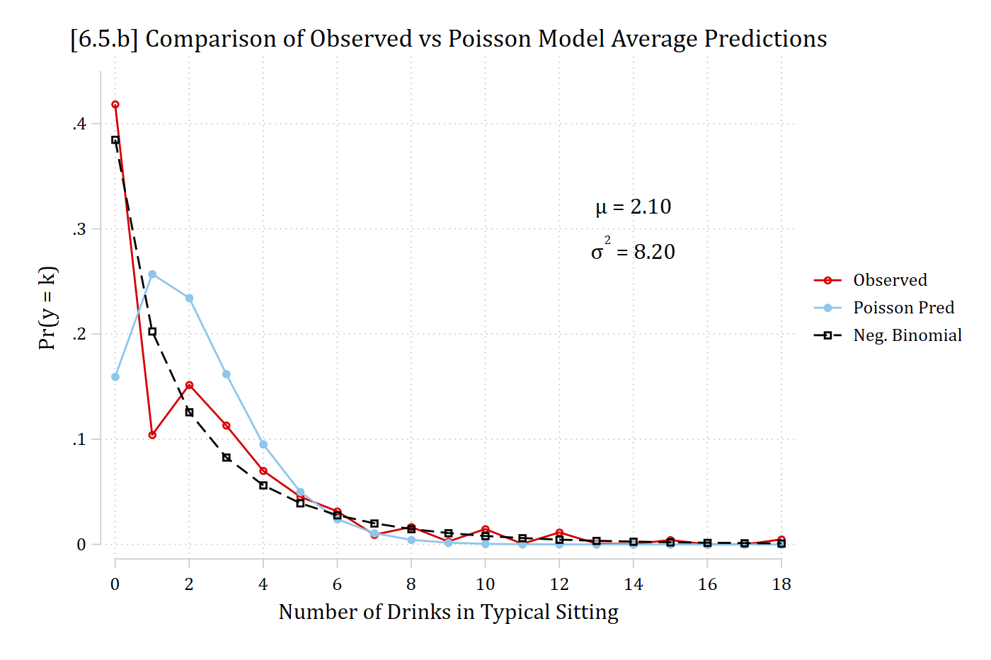
[6.5.b] Observed proportions of each number of drinks with the average predicted probabilities from the Poisson and negative binomial models: the negative binomial predicts about 38% at 0 drinks, close to the 42% observed, while the Poisson predicts about 16%; the negative binomial also tracks the observed proportions at 1 to 4 drinks much better.

library(tidyr)           # reshape data: pivot_longer()

# 6.5.b - Observed proportions and average predicted probabilities of each count
meanpred <- data.frame(k = 0:18) |>
  mutate(Observed = sapply(k, function(j) mean(ah4$drinktime == j)),
    "Poisson Pred" = sapply(k, function(j) mean(dpois(j, fitted(pmod)))),
    "Neg. Binomial" = sapply(k, function(j)
      mean(dnbinom(j, size = nbmod$theta, mu = fitted(nbmod))))) |>
  pivot_longer(-k, names_to = "type", values_to = "pr") |>
  mutate(type = factor(type, levels = c("Observed", "Poisson Pred", "Neg. Binomial")))

ggplot(meanpred, aes(x = k, y = pr, color = type)) +
  geom_line() + geom_point() +
  annotate("text", x = 14, y = .3, label = 'mu == "2.10"', parse = TRUE) +
  annotate("text", x = 14, y = .27, label = 'sigma^2 == "8.20"', parse = TRUE) +
  scale_x_continuous(breaks = seq(0, 18, 2)) +
  scale_y_continuous(breaks = seq(0, .4, .1), limits = c(0, .45)) +
  labs(title = "[6.5.b] Comparison of Observed vs Poisson Model Average Predictions",
    x = "Number of Drinks in Typical Sitting", y = "Pr(y = k)", color = NULL)

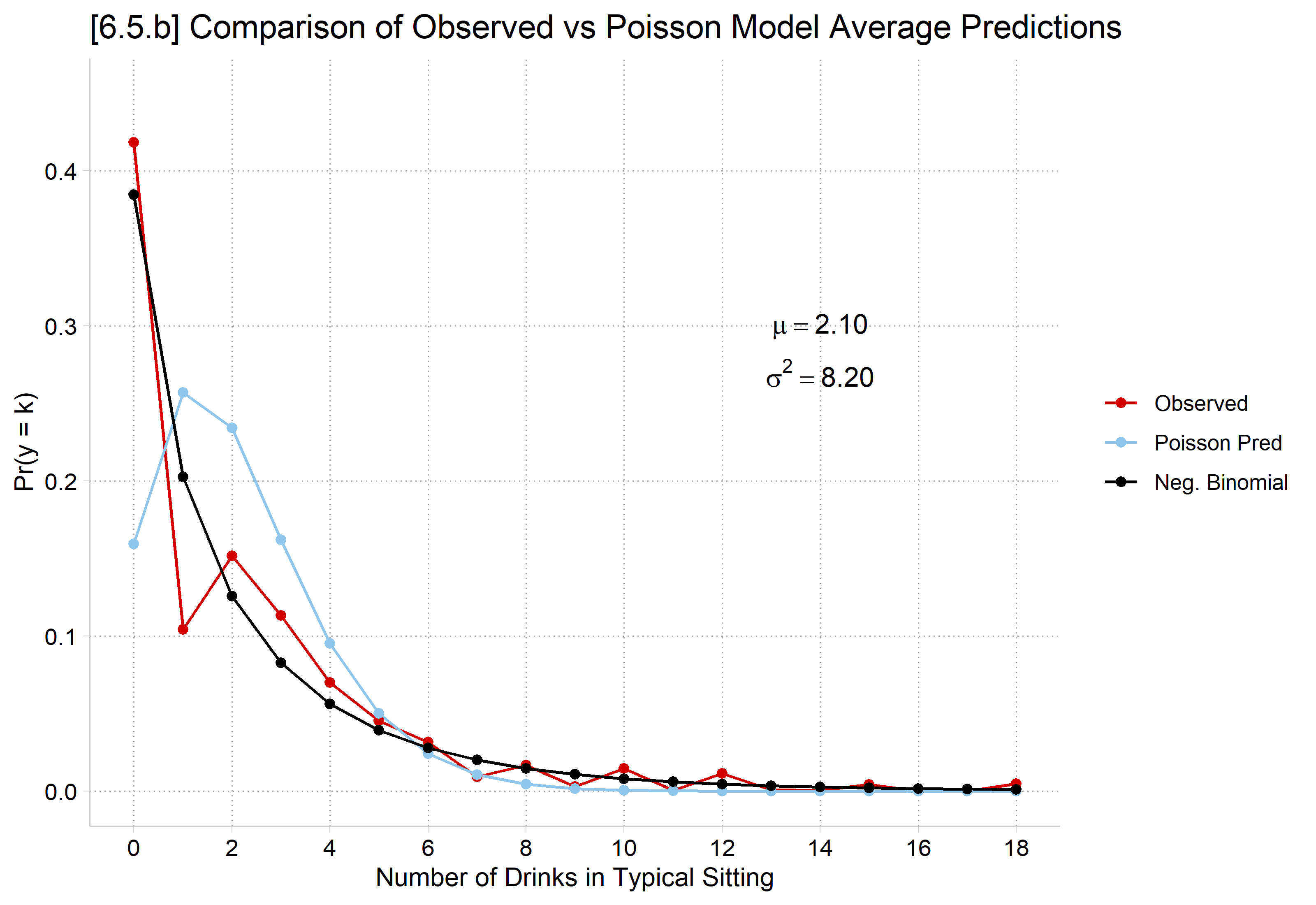
[6.5.b] Observed proportions of each number of drinks with the average predicted probabilities from the Poisson and negative binomial models: the negative binomial predicts about 38% at 0 drinks, close to the 42% observed, while the Poisson predicts about 16%; the negative binomial also tracks the observed proportions at 1 to 4 drinks much better.

Negative binomial does a noticeably better job at modeling the observed data

Back to top