5.0 Ordinal Outcomes

*Can assign values (e.g., 1 to 6) to these items but only ordering is meaningful; spacing between categories is not meaningful/consistent

What does ordinality mean?

• An ordinal variable has:
  • Categories ordered on a single dimension
  • Unknown distances between categories

• An ordinal model is defined by the nature of the relationship between independent variables and outcomes (Anderson 1984)
  • That is, the IVs are associated with a DV in an ordinal relationship
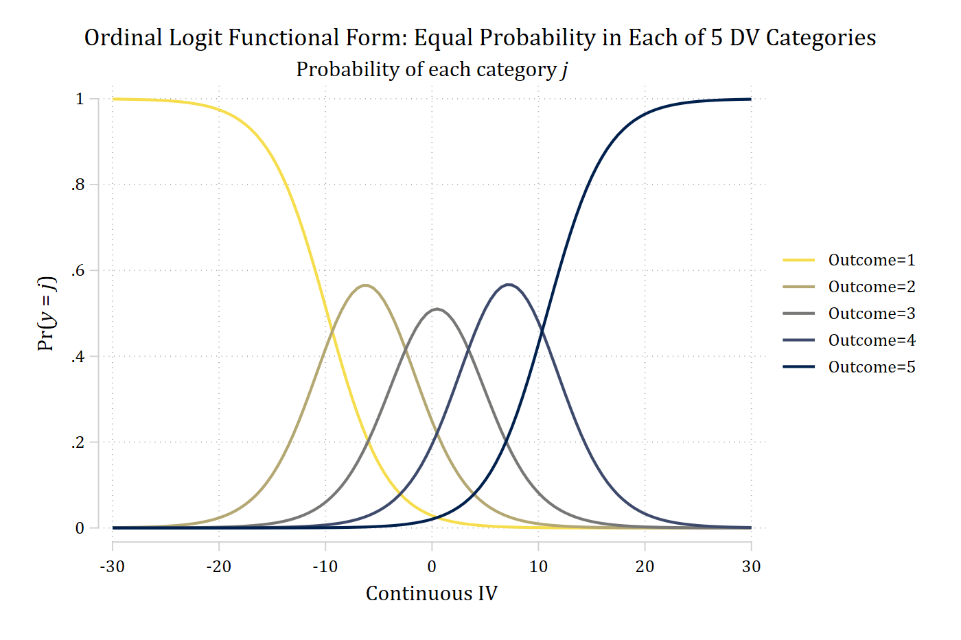
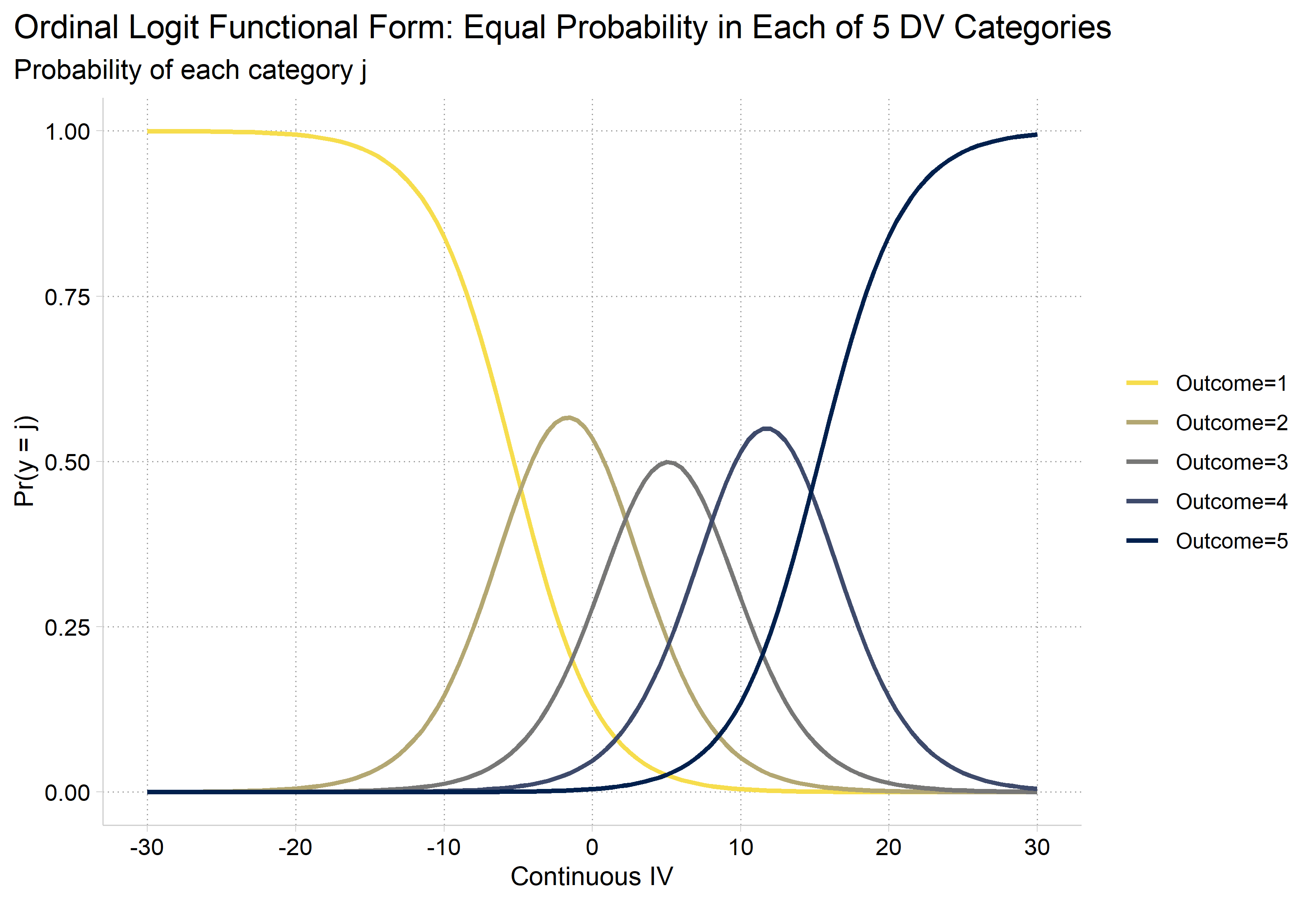
• Anderson (1984) shows that the following pattern between an ordinal DV and continuous IV must be found for the relationship to be ordinal (see below)
  • I.e., This is the relationship assumed by an ordinal model

Stata

*Simulate data to show ordinal model
clear
set seed 30004
set obs 2000

Number of observations (_N) was 0, now 2,000.

matrix P = (1, 0.2 \ 0.2, 1) // Small correlation
corr2data x1 x2, n(2000) cov(P)
gen c = rnormal(0,10)
gen b = c
replace b = 0 in 1/1000

(1,000 real changes made)

replace b = 1 in 1001/2000

(1,000 real changes made)

gen ystar = 0 + 0.2*(c) + 2*(b) + rnormal()
*Cut ystar into five categories with equal numbers of observations
xtile y = ystar, nq(5)
** Ordinal Models **
// Equal distribution in each outcome category //
qui ologit y c.c i.b x1 x2
*Pr(probs)
qui margins, at(c=(-30(.5)30)) atmeans
marginsplot, noci plotopts(msym(none) lwidth(medthick) lpat(solid)) ///
    xlab(-30(10)30) xtitle("Continuous IV") ytitle("Pr({it:y} = {it:j})") ///
    title("Ordinal Logit Functional Form: Equal Probability in Each of 5 DV Ca
tegories", size(medium)) ///
    subtitle("Probability of each category {it:j}") ///
    scheme(cleanplots5)

Variables that uniquely identify margins: c

R

library(haven)           # import Stata data and labels
library(dplyr)           # data manipulation
library(ggplot2)         # graphs
library(MASS)            # ordinal logit: polr(); mvrnorm()
library(marginaleffects) # predictions and marginal effects
library(cleanplots)      # graph scheme
cleanplots_defaults()

# Simulate data to show ordinal model
# (R's random numbers differ from Stata's, so the estimates differ a little)
set.seed(30004)
n <- 2000
sim <- as.data.frame(mvrnorm(n, mu = c(0, 0), Sigma = matrix(c(1, .2, .2, 1), 2),
  empirical = TRUE))  # x1 and x2 with a small correlation
names(sim) <- c("x1", "x2")
sim <- sim |>
  mutate(c = rnorm(n, 0, 10),
    b = rep(0:1, each = n / 2),
    ystar = 0 + 0.2 * c + 2 * b + rnorm(n),
    y = factor(ntile(ystar, 5)))  # five categories with equal numbers of observations

# Equal distribution in each outcome category
simmod <- polr(y ~ c + b + x1 + x2, data = sim, Hess = TRUE)

# Pr(probs) with the other IVs at their means
pr_sim <- predictions(simmod, newdata = datagrid(c = seq(-30, 30, .5)))

ggplot(pr_sim, aes(x = c, y = estimate, color = group)) +
  geom_line(linewidth = 1) +
  scale_color_viridis_d(option = "cividis", end = .95, direction = -1,
    labels = paste0("Outcome=", 1:5)) +
  scale_x_continuous(breaks = seq(-30, 30, 10)) +
  labs(title = "Ordinal Logit Functional Form: Equal Probability in Each of 5 DV Categories",
    subtitle = "Probability of each category j",
    x = "Continuous IV", y = "Pr(y = j)", color = NULL) +
  theme(plot.title.position = "plot")

Note that cumulatively the five Pr(y = j) must sum to one at any given value of x

Is the outcome ordered?

• Because values can be ordered does not mean it is substantively meaningful to order categories
• A variable can be partially ordered such as SA, A, D, SD, Don’t Know
• A variable can be ordered on multiple dimensions
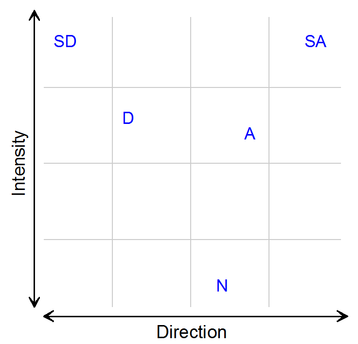
  • Likert scale items* usually reflect two dimensions, not one

Stats tip: Ordinal \(\neq\) Likert. Likert is a more specific category, referring to a “strongly disagree” to “strongly agree” set of response options. The name comes from the scale’s inventor, Rensis Likert.

Strongly Disagree	Disagree	Neutral	Agree	Strongly Agree
1	2	3	4	5

Multiple ordering of a Likert scale

How a given independent variable influences the outcome depends on the relationship of interest. For example, some opinions might show partisan differences; these could possibly be that liberals and conservatives differ on how much they agree or disagree about something, but also possibly how likely they are to report strong opinions about something (or both)

Ordinal is not interval

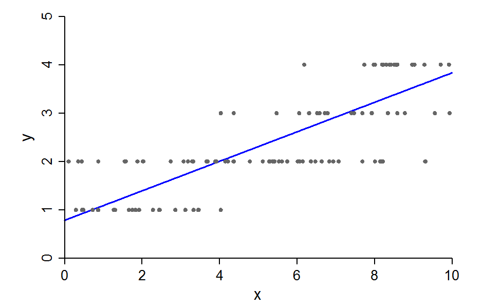
• Researchers often treat ordinal variables as interval (e.g., in a linear regression)
  • Doing this treats the category spacing as real and meaningful information
    • In addition, we lose any ability to examine how things are associated with each individual outcome category

When can I treat ordinal as continuous?

• Linear regression for an ordinal DV imposes equidistance spacing among outcome categories
  • Can bias conclusions (see Liddell and Kruschke 2018)
  • Model assumptions (e.g., homoscedasticity of residuals) are likely violated which can bias your standard error estimates/significance testing
  • Imposition of linearity can lead to spurious interaction effects (Rohrer and Arslan 2021)
• While there are no hard and fast rules, some methodological work (Rhemtulla et al. 2012; McNeish and Savord 2025) suggests:
  • If you have 4 or fewer categories you should use an ordinal model
  • If you have ≥ 5 categories, can usually treat as continuous if outcome is ≈normally distributed
  • But, with complications like (a) outcome is skewed and/or (b) have a multilevel or longitudinal model, need 7+ categories to treat as continuous

Effects of assuming wrong level of measurement

Model choice (assumed level of DV for analysis)	True level of DV: Nominal	Ordinal	Continuous*
Nominal	Ideal	Inefficient	Inefficient
Ordinal	Biased	Ideal	Inefficient
Continuous	Biased	Biased	Ideal

*I am not distinguishing between interval and ratio variables here

• An ordinal model will always be more accurate than treating outcomes as continuous (but sometimes with small benefit)
  • Do you want a model that is always right, or one that is sometimes right and sometimes notably biased? (Liddell and Kruschke 2018)
• To examine dynamics for specific outcome categories, must use an ordinal model

Stata

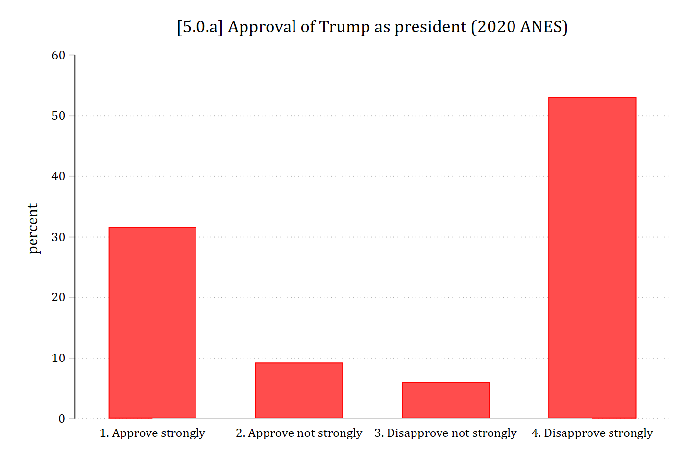
*2020 ANES
use "https://tdmize.github.io/data/data/cda_anes", clear

(American National Election Study 2020 - Pre-election | CDA | 2021-09-26)

*Distribution of ordinal DV
graph bar, over(trumpapprove4) ylab(0(10)60) ///
    title("[5.0.a] Approval of Trump as president (2020 ANES)")

R

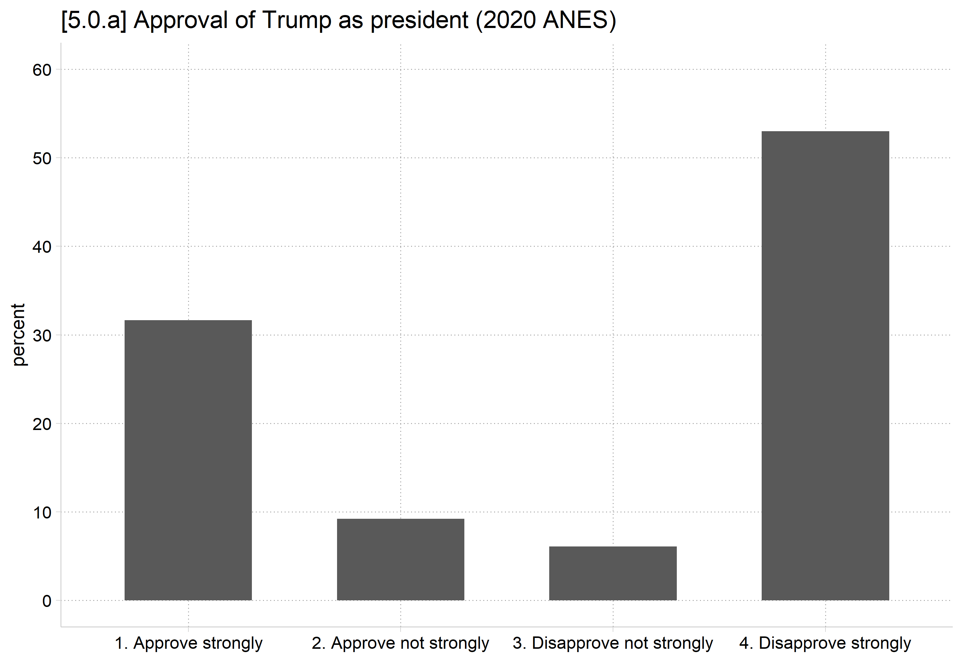
# 2020 ANES
anes <- read_dta("https://tdmize.github.io/data/data/cda_anes.dta")

# Distribution of ordinal DV
anes |>
  filter(!is.na(trumpapprove4)) |>
  count(trumpapprove4 = as_factor(trumpapprove4)) |>
  mutate(percent = 100 * n / sum(n)) |>
  ggplot(aes(x = trumpapprove4, y = percent)) +
  geom_col(width = .6) +
  scale_x_discrete(drop = TRUE) +
  scale_y_continuous(breaks = seq(0, 60, 10), limits = c(0, 60)) +
  labs(title = "[5.0.a] Approval of Trump as president (2020 ANES)", x = NULL)