4.5 Conditional Odds Ratios (ORs)

Consider an example I simulated below…

*Show simulation of mlogit where MEs and coefs diverge
clear
set seed 3704
set obs 5000
Number of observations (_N) was 0, now 5,000.
gen x1 = rnormal()
gen x2 = rnormal()
gen xb1 = ln(.5) + ln(1.5)*x1 + ln(.5)*x2
gen xb2 = ln(2) + ln(.33)*x1 + ln(2)*x2
gen p1 = 1 / ( 1 + exp(xb2) )
gen p2 = exp(xb1) / ( 1 + exp(xb1) + exp(xb2) )
gen p3 = exp(xb2) / ( 1 + exp(xb1) + exp(xb2) )
gen u = runiform()
gen y = cond(u < p1, 1, ///
    cond(u < p1 + p2, 2, 3 ))
qui mlogit y x1 x2, base(1) rrr
est store simmod
*4.5.a
qui margins, at(x2=(-2.5(.1)2.5))
marginsplot, recastci(rarea) ciopt(col(gs14)) ///
    plotopts(lwid(medthick) msym(none)) xlab(-2.5(1)2.5) ///
    xtitle("Continuous IV") ytitle("Pr(Outcome)") ///
    title("[4.5.a] Pr(Outcome) from Simulated Multinomial Logit Model", size(m
edlarge))
Variables that uniquely identify margins: x2

[4.5.a] Predicted probabilities of three outcomes across the continuous IV from -2.5 to 2.5: Pr(outcome 1) falls from about 0.57 to 0.09, Pr(outcome 2) falls from about 0.35 to 0.02, and Pr(outcome 3) rises from about 0.08 to 0.89.

library(haven)           # import Stata data and labels
library(dplyr)           # data manipulation
library(ggplot2)         # graphs
library(nnet)            # multinomial logit: multinom()
library(marginaleffects) # predictions and marginal effects
library(cleanplots)      # graph scheme
cleanplots_defaults()

# Center changes in continuous IVs on each observation's value
options(marginaleffects_contrast_direction = "center")

# Show simulation of a multinomial logit where MEs and coefs diverge
# (R's random numbers differ from Stata's, so the estimates differ a little)
set.seed(3704)
n <- 5000
sim <- data.frame(x1 = rnorm(n), x2 = rnorm(n)) |>
  mutate(xb1 = log(.5) + log(1.5) * x1 + log(.5) * x2,
    xb2 = log(2) + log(.33) * x1 + log(2) * x2,
    p1 = 1 / (1 + exp(xb2)),
    p2 = exp(xb1) / (1 + exp(xb1) + exp(xb2)),
    p3 = exp(xb2) / (1 + exp(xb1) + exp(xb2)),
    u = runif(n),
    y = factor(case_when(u < p1 ~ 1, u < p1 + p2 ~ 2, TRUE ~ 3)))

simmod <- multinom(y ~ x1 + x2, data = sim, trace = FALSE)

# 4.5.a
plot_predictions(simmod, by = c("x2", "group"),
  newdata = datagrid(x2 = seq(-2.5, 2.5, .1), grid_type = "counterfactual")) +
  scale_x_continuous(breaks = seq(-2.5, 2.5, 1)) +
  labs(title = "[4.5.a] Pr(Outcome) from Simulated Multinomial Logit Model",
    x = "Continuous IV", y = "Pr(Outcome)", color = "Outcome", fill = "Outcome")

[4.5.a] Predicted probabilities of three outcomes across the continuous IV from -2.5 to 2.5: Pr(outcome 1) falls from about 0.57 to 0.09, Pr(outcome 2) falls from about 0.35 to 0.02, and Pr(outcome 3) rises from about 0.08 to 0.89.

Write down your general interpretation of the effect of the continuous IV (x2)

Comparing MEs and coefficients in multinomial logit

  • Below are the AMEs for x2 (from the model graphed above):
*AMEs for +SD for x2
mecompare x2, amount(sd) model(simmod)
Predicting: Pr(y)
Marginal effects (N_simmod=5000)

                                 |  ME #   Estimate         SE      P>|z|
---------------------------------+---------------------------------------
x2 + SD (centered)               |                                       
              Outcome 1 - simmod |     1     -0.114      0.006      0.000
              Outcome 2 - simmod |     2     -0.071      0.005      0.000
              Outcome 3 - simmod |     3      0.186      0.005      0.000
# AMEs for +SD for x2
avg_comparisons(simmod, variables = list(x2 = sd(sim$x2)))

 Group Estimate Std. Error     z Pr(>|z|)     S   2.5 %  97.5 %
     1  -0.1190    0.00564 -21.1   <0.001 326.3 -0.1301 -0.1080
     2  -0.0731    0.00488 -15.0   <0.001 166.2 -0.0826 -0.0635
     3   0.1921    0.00443  43.3   <0.001   Inf  0.1834  0.2008

Term: x2
Type: probs
Comparison: +0.99401597047263
  • How do these compare to your descriptions of the effect of x2 that you wrote down based only on the graph shown above?
*All ORs for x2
est restore simmod
(results simmod are active now)
listcoef x2
mlogit (N=5000): Factor change in the odds of y 

Variable: x2 (sd=0.999)
------------------------------------------------------------------------------
                             |         b        z    P>|z|       e^b   e^bStdX
-----------------------------+------------------------------------------------
1            vs 2            |    0.1858    3.776    0.000     1.204     1.204
1            vs 3            |   -1.2784  -25.272    0.000     0.278     0.279
2            vs 1            |   -0.1858   -3.776    0.000     0.830     0.831
2            vs 3            |   -1.4642  -24.046    0.000     0.231     0.232
3            vs 1            |    1.2784   25.272    0.000     3.591     3.584
3            vs 2            |    1.4642   24.046    0.000     4.324     4.315
------------------------------------------------------------------------------
# All contrasts among the outcomes: refit the model with each outcome
# category as the base/reference category
all_contrasts <- function(model, term) {
  data <- eval(model$call$data)
  y <- all.vars(formula(model))[1]
  out <- lapply(model$lev, function(ref) {
    data[[y]] <- relevel(data[[y]], ref = ref)
    s <- summary(update(model, data = data))
    b <- s$coefficients[, term]
    z <- b / s$standard.errors[, term]
    data.frame(contrast = paste(rownames(s$coefficients), "vs", ref),
      b = round(b, 4), z = round(z, 3), p = round(2 * pnorm(-abs(z)), 3),
      exp_b = round(exp(b), 3), row.names = NULL)
  })
  do.call(rbind, out)
}

# All ORs for x2
all_contrasts(simmod, "x2")
  contrast       b       z     p exp_b
1   2 vs 1 -0.1594  -3.203 0.001 0.853
2   3 vs 1  1.3261  26.197 0.000 3.767
3   1 vs 2  0.1594   3.202 0.001 1.173
4   3 vs 2  1.4856  24.529 0.000 4.418
5   1 vs 3 -1.3262 -26.197 0.000 0.265
6   2 vs 3 -1.4856 -24.530 0.000 0.226
  • Note, column “b” is the log-odds; column “e^b” is exp(b) which are the conditional odds ratios
  • To start, let’s examine the effects for category 3 (odds of category 3 compared to odds of category 2 and category 1)
    • Do these match your general impressions of the effects of x2?
  • What about the effect of category 1 vs 2—the odds of category 1 compared to category 2?
    • Do these match your general impressions of the effects of x2?

Multinomial logit is a set of binary logits that are simultaneously estimated

Recall back to our example of political views (Conservative, Moderate, Liberal):

  • L vs M using nL + nM observations

\[\ln\left[\frac{\Pr(L\,|\,\mathbf{x}_{i})}{\Pr(M\,|\,\mathbf{x}_{i})}\right] = \beta_{0,L|M} + \boldsymbol{\beta}_{X,L|M}\,\mathbf{x}_{i}\]

Interpretation: For a unit increase in xk the odds of category L versus category M change by a factor of exp(βk, L|M), conditional on not being in any other categories

  • The “conditional on not being in any other categories” part is important and what distinguishes an exponentiated coefficient in multinomial logit from a true odds ratio from binary logit
    • In the example above only the observations in categories L or M are being compared
    • Observations in category C are not used—the odds ratio for L vs M is conditional on the observation not being in category C

Odds ratios (ORs) vs conditional ORs

  • Consider a binary outcome conservative/not and gender (woman=1) as an IV

    Pr(conserv = 1 | woman = 0) = .3594

    Pr(conserv = 1 | woman = 1) = .2962

use "https://tdmize.github.io/data/data/cda_gss", clear
(cda_gss.dta |  GSS 1972-2021 CDA - Categorical Data Analysis | date created 202
> 3)
keep if year >= 2016 & year <= 2021
(59,599 observations deleted)
drop if missing(conserv, age, woman, race3, college, married, parent, faminc)
(1,421 observations deleted)
*Show that OR in binary logit = ratio of two risk ratios
tab conserv woman, col
+-------------------+
| Key               |
|-------------------|
|     frequency     |
| column percentage |
+-------------------+

                 |        Woman R
  Conservative R |       Men      Women |     Total
-----------------+----------------------+----------
Not Conservative |     2,280      3,003 |     5,283 
                 |     64.06      70.38 |     67.51 
-----------------+----------------------+----------
    Conservative |     1,279      1,264 |     2,543 
                 |     35.94      29.62 |     32.49 
-----------------+----------------------+----------
           Total |     3,559      4,267 |     7,826 
                 |    100.00     100.00 |    100.00 
gss <- read_dta("https://tdmize.github.io/data/data/cda_gss.dta")

gss <- gss |> filter(year >= 2016 & year <= 2021)

# Keep model variables; drop any missing data
gss <- gss[c("conserv", "polviews3", "age", "woman", "race3", "college",
  "married", "parent", "faminc", "employed")]
gss <- gss[complete.cases(gss[c("conserv", "age", "woman", "race3", "college",
  "married", "parent", "faminc")]), ]

# Treat binary/nominal variables as factors
gss <- gss |>
  mutate(across(c(polviews3, woman, race3, college, married, parent, employed), as_factor)) |>
  droplevels()

# Show that OR in binary logit = ratio of two risk ratios
table(as_factor(gss$conserv), gss$woman)
                  
                    Men Women
  Not Conservative 2280  3003
  Conservative     1279  1264
round(100 * prop.table(table(as_factor(gss$conserv), gss$woman), margin = 2), 2)  # column %
                  
                     Men Women
  Not Conservative 64.06 70.38
  Conservative     35.94 29.62

Odds ratios in binary logit

di "Odds of being conservative for women = " .2962 / (1 - .2962)
Odds of being conservative for women = .4208582
di "Odds of being conservative for men = " .3594 / (1 - .3594)
Odds of being conservative for men = .56103653
di "Odds ratio of women / men = " .4208582 / .56103653
Odds ratio of women / men = .75014402
logit conserv i.woman, or nolog
Logistic regression                                     Number of obs =  7,826
                                                        LR chi2(1)    =  35.21
                                                        Prob > chi2   = 0.0000
Log likelihood = -4916.995                              Pseudo R2     = 0.0036

------------------------------------------------------------------------------
     conserv | Odds ratio   Std. err.      z    P>|z|     [95% conf. interval]
-------------+----------------------------------------------------------------
       woman |
      Women  |      0.750      0.036   -5.932   0.000        0.682       0.825
       _cons |      0.561      0.020  -16.548   0.000        0.524       0.601
------------------------------------------------------------------------------
Note: _cons estimates baseline odds.
# Odds of being conservative for women
.2962 / (1 - .2962)
[1] 0.4208582
# Odds of being conservative for men
.3594 / (1 - .3594)
[1] 0.5610365
# Odds ratio of women / men
.4208582 / .56103653
[1] 0.750144
genmod <- glm(conserv ~ woman, data = gss, family = binomial(link = "logit"))
exp(cbind(OR = coef(genmod), confint.default(genmod)))
                   OR     2.5 %    97.5 %
(Intercept) 0.5609649 0.5238403 0.6007205
womanWomen  0.7503365 0.6824015 0.8250345

The odds ratio (OR) from a binary logit is the ratio of women to men’s odds

Nominal DVs and conditional ORs

tab polviews3 woman, col
+-------------------+
| Key               |
|-------------------|
|     frequency     |
| column percentage |
+-------------------+

   Political |
        View |        Woman R
  Categories |       Men      Women |     Total
-------------+----------------------+----------
     Liberal |     1,100      1,392 |     2,492 
             |     30.91      32.62 |     31.84 
-------------+----------------------+----------
    Moderate |     1,180      1,611 |     2,791 
             |     33.16      37.75 |     35.66 
-------------+----------------------+----------
Conservative |     1,279      1,264 |     2,543 
             |     35.94      29.62 |     32.49 
-------------+----------------------+----------
       Total |     3,559      4,267 |     7,826 
             |    100.00     100.00 |    100.00 
table(gss$polviews3, gss$woman)
              
                Men Women
  Liberal      1100  1392
  Moderate     1180  1611
  Conservative 1279  1264
round(100 * prop.table(table(gss$polviews3, gss$woman), margin = 2), 2)  # column %
              
                 Men Women
  Liberal      30.91 32.62
  Moderate     33.16 37.75
  Conservative 35.94 29.62
  • Recall from above the OR for gender (woman=1): .4208582 / .56103653 = .75014402

Conditional odds ratios / “relative risk ratios”

mlogit polviews3 i.woman, base(1) rrr nolog cformat(%6.4f)
Multinomial logistic regression                         Number of obs =  7,826
                                                        LR chi2(2)    =  37.07
                                                        Prob > chi2   = 0.0000
Log likelihood = -8569.4951                             Pseudo R2     = 0.0022

------------------------------------------------------------------------------
   polviews3 |        RRR   Std. err.      z    P>|z|     [95% conf. interval]
-------------+----------------------------------------------------------------
Liberal      |  (base outcome)
-------------+----------------------------------------------------------------
Moderate     |
       woman |
      Women  |     1.0789     0.0600    1.364   0.172       0.9674      1.2032
       _cons |     1.0727     0.0450    1.675   0.094       0.9881      1.1646
-------------+----------------------------------------------------------------
Conservative |
       woman |
      Women  |     0.7810     0.0442   -4.370   0.000       0.6990      0.8725
       _cons |     1.1627     0.0478    3.666   0.000       1.0727      1.2603
------------------------------------------------------------------------------
Note: _cons estimates baseline relative risk for each outcome.
pol3mod <- multinom(polviews3 ~ woman, data = gss, trace = FALSE)
exp(coef(pol3mod))
             (Intercept) womanWomen
Moderate        1.072727   1.078865
Conservative    1.162727   0.780962
  • The conditional OR for women is 0.7810 in the conservative panel—which does not match the OR of 0.750 we calculated above. Why do you think this is?

* Quick terminology note: Stata uses the term “relative risk ratio” (rationale for term here) which is a synonym for conditional odds ratio; this is the exponentiated regression coefficient

Calculating conditional ORs / relative risk ratios (RRRs)

di "Women: pr(conserv) conditional on not being moderate = " .2962 / (.2962 + 
.3262)
Women: pr(conserv) conditional on not being moderate = .47589974
di "Men: pr(conserv) conditional on not being moderate = " .3594 / (.3594 + .3
091)
Men: pr(conserv) conditional on not being moderate = .53762154
di "Women: Odds(conserv) conditional on not being moderate = " .47589974 / (1 
- .47589974)
Women: Odds(conserv) conditional on not being moderate = .90803187
di "Men: Odds(conserv) conditional on not being moderate = " .53762154 / (1 - 
.53762154)
Men: Odds(conserv) conditional on not being moderate = 1.1627305
di "Odds ratio of women / men conditional on not being moderate = " .90803187 
/ 1.1627305
Odds ratio of women / men conditional on not being moderate = .78094784
# Women: pr(conserv) conditional on not being moderate
.2962 / (.2962 + .3262)
[1] 0.4758997
# Men: pr(conserv) conditional on not being moderate
.3594 / (.3594 + .3091)
[1] 0.5376215
# Women: Odds(conserv) conditional on not being moderate
.47589974 / (1 - .47589974)
[1] 0.9080319
# Men: Odds(conserv) conditional on not being moderate
.53762154 / (1 - .53762154)
[1] 1.162731
# Odds ratio of women / men conditional on not being moderate
.90803187 / 1.1627305
[1] 0.7809478

Remember that the coefficients mlogit reports are conditional on not being in other categories—here, the coefficient in conservative panel is for Conservative vs Liberal (the base/reference category), conditional on not being moderate

Interpreting conditional ORs / RRRs

  • Because of this “conditional” nature of the coefficients in multinomial logit, it is not strictly appropriate to refer to them as odds ratios
    • Some call these “conditional odds ratios” (an interesting discussion here)
    • Others conceptualize them as “relative risk ratios” (Stata’s term, explained here)—TLDR: mathematically a ratio of two risk ratios (conditional on not being in other categories) is equivalent to a conditional odds ratio
    • Long and Freese 2014 refer to them simply as odds ratios
      • Within sociology, referring to them as “odds ratios” is not problematic and you generally will be understood
      • May not be the case in other fields
        • Within or outside of sociology, it cannot hurt to note your understanding of this distinction in your Analytic Strategy section of your paper. E.g., Feel free to copy this for your needs:

I report exponentiated coefficients from the multinomial logit models, which represent conditional odds ratios (AKA relative risk ratios)—referred to simply as “odds ratios” in what follows (see Long and Freese 2014).

Interpreting ORs in multinomial logit

  • In Stata, the SPost command listcoef will calculate ORs for all contrasts for you
qui mlogit polviews3 c.age i.woman i.race3 i.college ///
    i.married i.parent c.faminc i.employed
est store pol3mod
listcoef age
mlogit (N=7823): Factor change in the odds of polviews3 

Variable: age (sd=17.361)
------------------------------------------------------------------------------
                             |         b        z    P>|z|       e^b   e^bStdX
-----------------------------+------------------------------------------------
Liberal      vs Moderate     |    0.0010    0.518    0.604     1.001     1.017
Liberal      vs Conservative |   -0.0130   -6.489    0.000     0.987     0.799
Moderate     vs Liberal      |   -0.0010   -0.518    0.604     0.999     0.983
Moderate     vs Conservative |   -0.0139   -7.329    0.000     0.986     0.785
Conservative vs Liberal      |    0.0130    6.489    0.000     1.013     1.252
Conservative vs Moderate     |    0.0139    7.329    0.000     1.014     1.274
------------------------------------------------------------------------------
  • In R, would need to refit model changing the reference outcome category
pol3mod <- multinom(polviews3 ~ age + woman + race3 + college + married + parent +
  faminc + employed, data = gss, trace = FALSE)

all_contrasts(pol3mod, "age")
                  contrast       b      z     p exp_b
1      Moderate vs Liberal -0.0010 -0.518 0.604 0.999
2  Conservative vs Liberal  0.0130  6.489 0.000 1.013
3      Liberal vs Moderate  0.0010  0.518 0.604 1.001
4 Conservative vs Moderate  0.0139  7.329 0.000 1.014
5  Liberal vs Conservative -0.0130 -6.489 0.000 0.987
6 Moderate vs Conservative -0.0139 -7.329 0.000 0.986

Each contrast appears twice (e.g., Liberal vs Moderate and Moderate vs Liberal), so half of the coefficients and significance tests are redundant; there are only three unique ORs. Which direction of the contrast to interpret depends on your research question, but there is no reason to interpret both

Interpreting ORs in multinomial logit: continuous IV

For a one year increase in age, the odds of identifying as conservative compared to moderate increase by a factor of 1.014 (holding all else constant)

For a one-year increase in age, the odds of identifying as conservative instead of liberal increase by a factor of 1.013 (all else equal)

Age has no significant effect on the odds of identifying as liberal compared to moderate (p = ns)

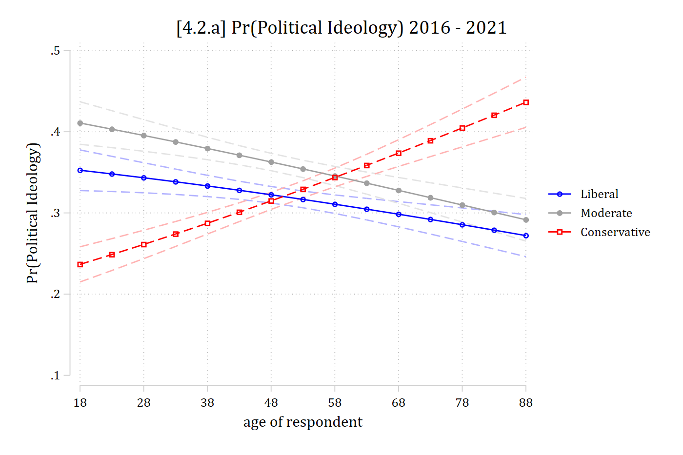
[4.2.a] Predicted probabilities of each political ideology by age with confidence intervals: Pr(liberal) falls from about 0.35 to 0.27, Pr(moderate) falls from about 0.41 to 0.29, and Pr(conservative) rises from about 0.24 to 0.44.

Do the ORs interpreted above tell the whole story? Would you be able to ascertain that age has a negative effect on the probability of identifying as moderate? A positive effect on the probability of identifying as conservative? Etc.

Interpreting ORs in multinomial logit: nominal IV

listcoef college
mlogit (N=7823): Factor change in the odds of polviews3 

Variable: 1.college (sd=0.485)
------------------------------------------------------------------------------
                             |         b        z    P>|z|       e^b   e^bStdX
-----------------------------+------------------------------------------------
Liberal      vs Moderate     |    0.9020   14.071    0.000     2.465     1.549
Liberal      vs Conservative |    0.7312   11.234    0.000     2.078     1.426
Moderate     vs Liberal      |   -0.9020  -14.071    0.000     0.406     0.645
Moderate     vs Conservative |   -0.1708   -2.602    0.009     0.843     0.920
Conservative vs Liberal      |   -0.7312  -11.234    0.000     0.481     0.701
Conservative vs Moderate     |    0.1708    2.602    0.009     1.186     1.086
------------------------------------------------------------------------------
all_contrasts(pol3mod, "collegeCollege Degree")
                  contrast       b       z     p exp_b
1      Moderate vs Liberal -0.9020 -14.071 0.000 0.406
2  Conservative vs Liberal -0.7312 -11.234 0.000 0.481
3      Liberal vs Moderate  0.9020  14.071 0.000 2.465
4 Conservative vs Moderate  0.1708   2.602 0.009 1.186
5  Liberal vs Conservative  0.7312  11.234 0.000 2.078
6 Moderate vs Conservative -0.1708  -2.602 0.009 0.843

For those with college degrees, the odds of identifying as liberal are 2.465 times higher than the odds of identifying as moderate (compared to those without college degrees)

The odds of identifying as liberal over conservative increase by a factor of 2.078 for those with a college degree

The odds of identifying as conservative compared to moderate are 1.186 times higher for those with a college degree

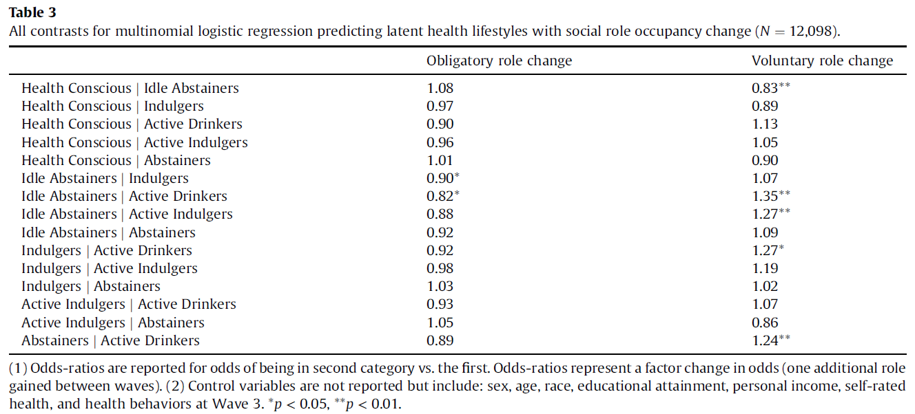
Table 3 from Mize (2017): odds ratios for all contrasts among five latent health lifestyles (Health Conscious, Idle Abstainers, Indulgers, Active Drinkers, Active Indulgers, Abstainers) for obligatory and voluntary role change; for example, Health Conscious versus Idle Abstainers is 1.08 for obligatory role change and 0.83 (p < 0.01) for voluntary role change.

“… the first row of the table indicates that obligatory role change does not distinguish between membership in the Idle Abstainer and Health Conscious lifestyle at Wave 4 (OR = 1.08, ns), but that gaining an additional voluntary role between waves is associated with lower odds of being in the Idle Abstainer lifestyle compared to being in the Health Conscious lifestyle (OR = 0.83, 95% CI [0.73, 0.93]).” (Mize 2017)
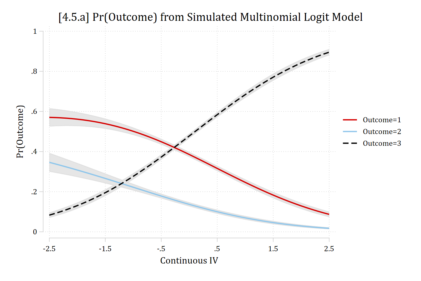
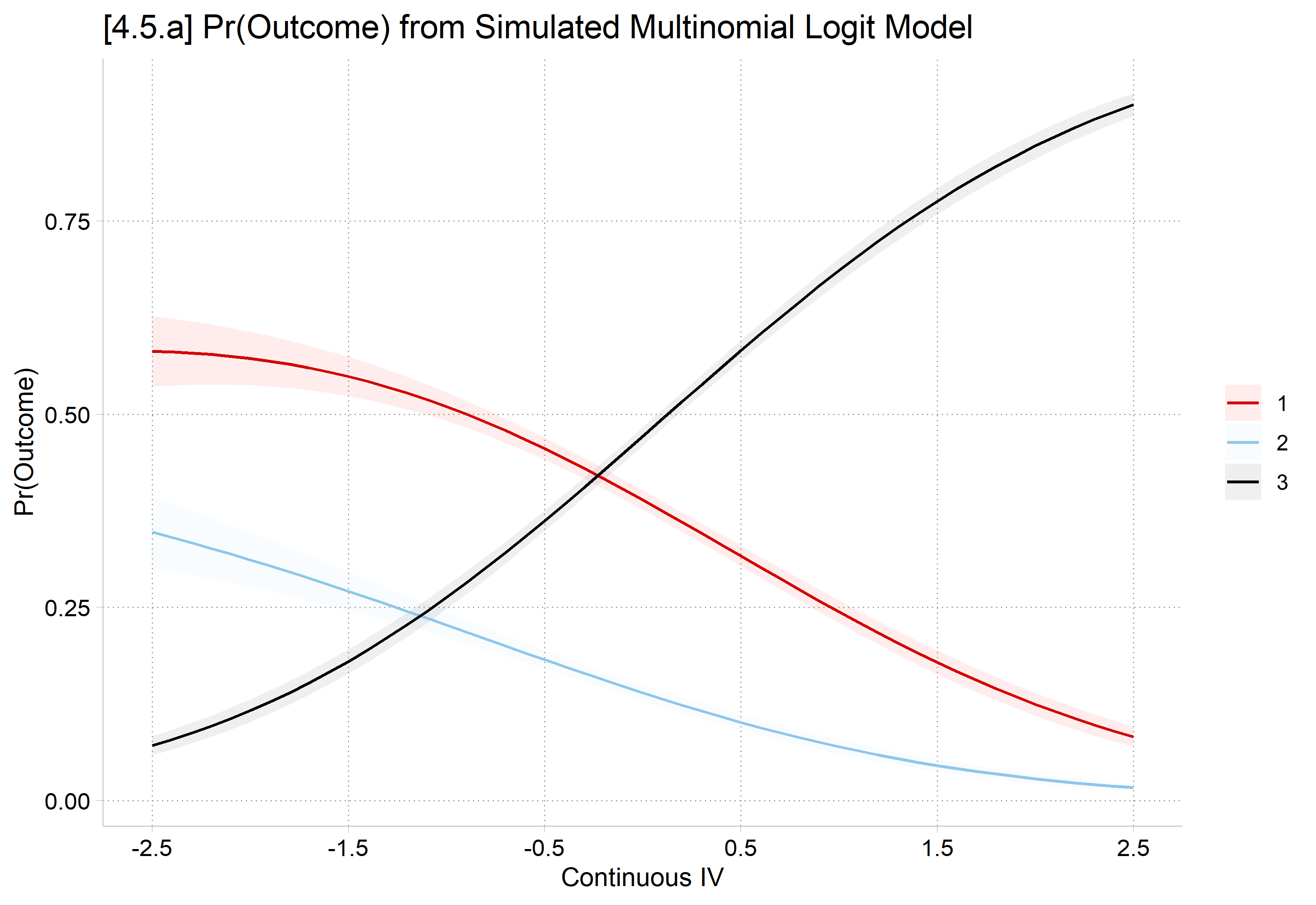
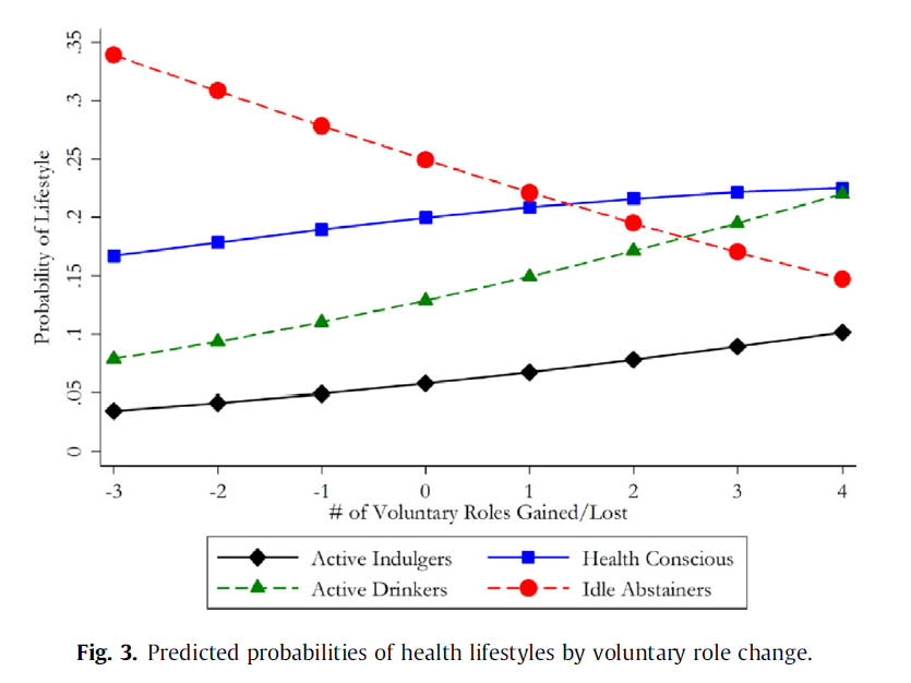
Figure 3 from Mize (2017): predicted probabilities of health lifestyles by the number of voluntary roles gained or lost, from -3 to 4: Idle Abstainers falls from about 0.34 to 0.15, Health Conscious rises from about 0.17 to 0.22, Active Drinkers rises from about 0.08 to 0.22, and Active Indulgers rises from about 0.03 to 0.10.

Back to top