2.7 Categorical Independent Variables
Ordinal independent variables
- Independent variables can be entered into a regression model one of two ways:
- Continuous
- Nominal (n.b., binary is nominal but with only 2 categories)
- For an ordinal IV, you must choose how to enter it (ordinal is not an option)
Continuous vs nominal specifications
- A continuous specification is simpler
- E.g., For a 5-category ordinal IV only need to estimate 1 coefficient
- A nominal is more complicated but always more accurate*
- If entering as nominal, need 4 coefficients (representing 4 categories and one omitted reference category)
- 4 coefficients will always provide a somewhat better fit* than 1
- Which should you choose? Try both:
- If inferences are very similar, choose the simpler specification (continuous)
- If inferences diverge, choose the more complicated but more accurate specification (nominal)
*We will cover how to provide a significance test of this in the Testing section. But R2 will always be same or higher in nominal specification (even if not significantly different)
The examples use the 2020 American National Election Studies (ANES):
use "https://tdmize.github.io/data/data/cda_anes", clear(American National Election Study 2020 - Pre-election | CDA | 2021-09-26)drop if missing(feel_trump, age, hhincome, woman, lgb, race4, ///
educ, relimport, wrongtrack)(1,125 observations deleted)regress feel_trump c.relimport i.educ age hhincome i.woman ///
i.lgb i.race4 i.wrongtrack Source | SS df MS Number of obs = 7,155
-------------+---------------------------------- F(13, 7141) = 506.04
Model | 5562481.5 13 427883.192 Prob > F = 0.0000
Residual | 6038073.21 7,141 845.550093 R-squared = 0.4795
-------------+---------------------------------- Adj R-squared = 0.4786
Total | 11600554.7 7,154 1621.54804 Root MSE = 29.078
-------------------------------------------------------------------------------
feel_trump | Coefficient Std. err. t P>|t| [95% conf. interval]
--------------+----------------------------------------------------------------
relimport | -5.949 0.249 -23.879 0.000 -6.438 -5.461
|
educ |
2. High sc.. | 1.915 1.851 1.035 0.301 -1.713 5.543
3. Some po.. | 0.002 1.747 0.001 0.999 -3.422 3.426
4. Bachelo.. | -6.789 1.808 -3.755 0.000 -10.333 -3.244
5. Graduat.. | -11.486 1.880 -6.108 0.000 -15.173 -7.800
|
age | -0.051 0.021 -2.401 0.016 -0.093 -0.009
hhincome | -0.014 0.006 -2.501 0.012 -0.025 -0.003
|
woman |
Woman | -4.472 0.700 -6.392 0.000 -5.844 -3.101
|
lgb |
LGB | -10.331 1.409 -7.331 0.000 -13.093 -7.568
|
race4 |
Black | -24.256 1.274 -19.037 0.000 -26.754 -21.758
Hispanic | -11.116 1.230 -9.038 0.000 -13.527 -8.705
Other | -4.763 1.234 -3.861 0.000 -7.181 -2.345
|
wrongtrack |
Wrong track | -49.332 0.832 -59.312 0.000 -50.963 -47.702
_cons | 107.667 2.319 46.433 0.000 103.121 112.212
-------------------------------------------------------------------------------margins, at(relimport=(1(1)5)) saving(con_reli, replace)Predictive margins Number of obs = 7,155
Model VCE: OLS
Expression: Linear prediction, predict()
1._at: relimport = 1
2._at: relimport = 2
3._at: relimport = 3
4._at: relimport = 4
5._at: relimport = 5
------------------------------------------------------------------------------
| Delta-method
| Margin std. err. t P>|t| [95% conf. interval]
-------------+----------------------------------------------------------------
_at |
1 | 50.688 0.576 88.008 0.000 49.559 51.817
2 | 44.739 0.404 110.633 0.000 43.946 45.531
3 | 38.789 0.346 112.216 0.000 38.112 39.467
4 | 32.840 0.447 73.509 0.000 31.964 33.716
5 | 26.891 0.635 42.316 0.000 25.645 28.136
------------------------------------------------------------------------------
(file con_reli.dta not found)regress feel_trump i.relimport i.educ age hhincome i.woman ///
i.lgb i.race4 i.wrongtrack Source | SS df MS Number of obs = 7,155
-------------+---------------------------------- F(16, 7138) = 412.05
Model | 5569952.94 16 348122.059 Prob > F = 0.0000
Residual | 6030601.77 7,138 844.858752 R-squared = 0.4801
-------------+---------------------------------- Adj R-squared = 0.4790
Total | 11600554.7 7,154 1621.54804 Root MSE = 29.066
-------------------------------------------------------------------------------
feel_trump | Coefficient Std. err. t P>|t| [95% conf. interval]
--------------+----------------------------------------------------------------
relimport |
2. Very im.. | -6.789 1.037 -6.545 0.000 -8.823 -4.756
3. Moderat.. | -10.903 1.039 -10.496 0.000 -12.939 -8.867
4. A littl.. | -15.893 1.193 -13.320 0.000 -18.232 -13.554
5. Not imp.. | -24.797 1.063 -23.327 0.000 -26.881 -22.713
|
educ |
2. High sc.. | 2.052 1.851 1.109 0.268 -1.576 5.680
3. Some po.. | 0.169 1.747 0.097 0.923 -3.256 3.595
4. Bachelo.. | -6.614 1.809 -3.657 0.000 -10.160 -3.068
5. Graduat.. | -11.321 1.882 -6.016 0.000 -15.010 -7.632
|
age | -0.051 0.021 -2.395 0.017 -0.093 -0.009
hhincome | -0.014 0.006 -2.548 0.011 -0.025 -0.003
|
woman |
Woman | -4.465 0.699 -6.384 0.000 -5.836 -3.094
|
lgb |
LGB | -10.203 1.409 -7.240 0.000 -12.966 -7.441
|
race4 |
Black | -24.244 1.274 -19.034 0.000 -26.741 -21.747
Hispanic | -11.164 1.230 -9.074 0.000 -13.576 -8.752
Other | -4.751 1.233 -3.852 0.000 -7.168 -2.333
|
wrongtrack |
Wrong track | -49.298 0.832 -59.257 0.000 -50.929 -47.667
_cons | 101.470 2.272 44.660 0.000 97.016 105.924
-------------------------------------------------------------------------------margins, at(relimport=(1(1)5)) saving(nom_reli, replace)Predictive margins Number of obs = 7,155
Model VCE: OLS
Expression: Linear prediction, predict()
1._at: relimport = 1
2._at: relimport = 2
3._at: relimport = 3
4._at: relimport = 4
5._at: relimport = 5
------------------------------------------------------------------------------
| Delta-method
| Margin std. err. t P>|t| [95% conf. interval]
-------------+----------------------------------------------------------------
_at |
1 | 50.616 0.689 73.494 0.000 49.266 51.966
2 | 43.826 0.793 55.237 0.000 42.271 45.382
3 | 39.713 0.783 50.732 0.000 38.178 41.247
4 | 34.723 0.953 36.440 0.000 32.855 36.590
5 | 25.819 0.765 33.749 0.000 24.319 27.318
------------------------------------------------------------------------------
(file nom_reli.dta not found)combomarginsplot con_reli nom_reli, ///
labels("Continuous" "Nominal") xtitle("Importance of religion") ///
xlab(1 "Extremely" 2 "Very" 3 "Moderately" 4 "A little" 5 "Not at all") //
/
title("[2.7.a] Trump feeling thermometer by importance of religion", size(
medlarge)) ///
subtitle("Nominal vs continuous specification of {it:relimport}") Variables that uniquely identify margins: relimport _filenumber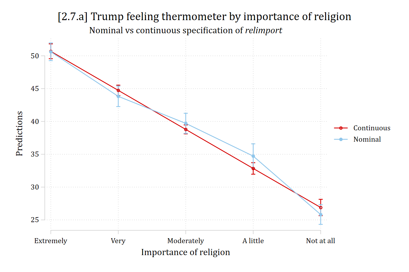
*These look similar enough to probably choose the continuous specification. But I would also do some statistical tests to decide (more in the Testing section of the class)
regress feel_trump c.educ i.relimport age hhincome i.woman ///
i.lgb i.race4 i.wrongtrack Source | SS df MS Number of obs = 7,155
-------------+---------------------------------- F(13, 7141) = 502.86
Model | 5544245.54 13 426480.426 Prob > F = 0.0000
Residual | 6056309.17 7,141 848.103791 R-squared = 0.4779
-------------+---------------------------------- Adj R-squared = 0.4770
Total | 11600554.7 7,154 1621.54804 Root MSE = 29.122
-------------------------------------------------------------------------------
feel_trump | Coefficient Std. err. t P>|t| [95% conf. interval]
--------------+----------------------------------------------------------------
educ | -4.097 0.341 -12.002 0.000 -4.767 -3.428
|
relimport |
2. Very im.. | -6.751 1.039 -6.496 0.000 -8.789 -4.714
3. Moderat.. | -11.021 1.040 -10.593 0.000 -13.061 -8.982
4. A littl.. | -15.969 1.195 -13.359 0.000 -18.312 -13.626
5. Not imp.. | -24.793 1.065 -23.279 0.000 -26.880 -22.705
|
age | -0.055 0.021 -2.574 0.010 -0.097 -0.013
hhincome | -0.016 0.006 -2.890 0.004 -0.027 -0.005
|
woman |
Woman | -4.329 0.700 -6.187 0.000 -5.701 -2.958
|
lgb |
LGB | -10.317 1.412 -7.309 0.000 -13.084 -7.550
|
race4 |
Black | -24.192 1.275 -18.967 0.000 -26.692 -21.691
Hispanic | -11.368 1.230 -9.238 0.000 -13.780 -8.955
Other | -4.881 1.235 -3.952 0.000 -7.302 -2.460
|
wrongtrack |
Wrong track | -49.475 0.833 -59.405 0.000 -51.108 -47.842
_cons | 112.350 1.860 60.408 0.000 108.704 115.996
-------------------------------------------------------------------------------margins, at(educ=(1(1)5)) saving(con_educ, replace)Predictive margins Number of obs = 7,155
Model VCE: OLS
Expression: Linear prediction, predict()
1._at: educ = 1
2._at: educ = 2
3._at: educ = 3
4._at: educ = 4
5._at: educ = 5
------------------------------------------------------------------------------
| Delta-method
| Margin std. err. t P>|t| [95% conf. interval]
-------------+----------------------------------------------------------------
_at |
1 | 49.467 0.887 55.754 0.000 47.728 51.207
2 | 45.370 0.588 77.196 0.000 44.218 46.522
3 | 41.273 0.370 111.613 0.000 40.548 41.998
4 | 37.175 0.401 92.604 0.000 36.388 37.962
5 | 33.078 0.647 51.122 0.000 31.810 34.347
------------------------------------------------------------------------------
(file con_educ.dta not found)regress feel_trump i.educ i.relimport age hhincome i.woman ///
i.lgb i.race4 i.wrongtrack Source | SS df MS Number of obs = 7,155
-------------+---------------------------------- F(16, 7138) = 412.05
Model | 5569952.94 16 348122.059 Prob > F = 0.0000
Residual | 6030601.77 7,138 844.858752 R-squared = 0.4801
-------------+---------------------------------- Adj R-squared = 0.4790
Total | 11600554.7 7,154 1621.54804 Root MSE = 29.066
-------------------------------------------------------------------------------
feel_trump | Coefficient Std. err. t P>|t| [95% conf. interval]
--------------+----------------------------------------------------------------
educ |
2. High sc.. | 2.052 1.851 1.109 0.268 -1.576 5.680
3. Some po.. | 0.169 1.747 0.097 0.923 -3.256 3.595
4. Bachelo.. | -6.614 1.809 -3.657 0.000 -10.160 -3.068
5. Graduat.. | -11.321 1.882 -6.016 0.000 -15.010 -7.632
|
relimport |
2. Very im.. | -6.789 1.037 -6.545 0.000 -8.823 -4.756
3. Moderat.. | -10.903 1.039 -10.496 0.000 -12.939 -8.867
4. A littl.. | -15.893 1.193 -13.320 0.000 -18.232 -13.554
5. Not imp.. | -24.797 1.063 -23.327 0.000 -26.881 -22.713
|
age | -0.051 0.021 -2.395 0.017 -0.093 -0.009
hhincome | -0.014 0.006 -2.548 0.011 -0.025 -0.003
|
woman |
Woman | -4.465 0.699 -6.384 0.000 -5.836 -3.094
|
lgb |
LGB | -10.203 1.409 -7.240 0.000 -12.966 -7.441
|
race4 |
Black | -24.244 1.274 -19.034 0.000 -26.741 -21.747
Hispanic | -11.164 1.230 -9.074 0.000 -13.576 -8.752
Other | -4.751 1.233 -3.852 0.000 -7.168 -2.333
|
wrongtrack |
Wrong track | -49.298 0.832 -59.257 0.000 -50.929 -47.667
_cons | 101.470 2.272 44.660 0.000 97.016 105.924
-------------------------------------------------------------------------------margins, at(educ=(1(1)5)) saving(nom_educ, replace)Predictive margins Number of obs = 7,155
Model VCE: OLS
Expression: Linear prediction, predict()
1._at: educ = 1
2._at: educ = 2
3._at: educ = 3
4._at: educ = 4
5._at: educ = 5
------------------------------------------------------------------------------
| Delta-method
| Margin std. err. t P>|t| [95% conf. interval]
-------------+----------------------------------------------------------------
_at |
1 | 43.157 1.658 26.033 0.000 39.907 46.407
2 | 45.209 0.877 51.563 0.000 43.490 46.928
3 | 43.326 0.592 73.214 0.000 42.166 44.486
4 | 36.543 0.685 53.343 0.000 35.200 37.885
5 | 31.836 0.817 38.990 0.000 30.235 33.437
------------------------------------------------------------------------------
(file nom_educ.dta not found)combomarginsplot con_educ nom_educ, ///
labels("Continuous" "Nominal") ///
xlab(1 "< High School" 2 "High School" 3 "Some College" 4 "College Degree"
5 "Grad+") ///
title("[2.7.b] Trump feeling thermometer by educational attainment", size(
medlarge)) ///
subtitle("Nominal vs continuous specification of {it:education}") Variables that uniquely identify margins: educ _filenumber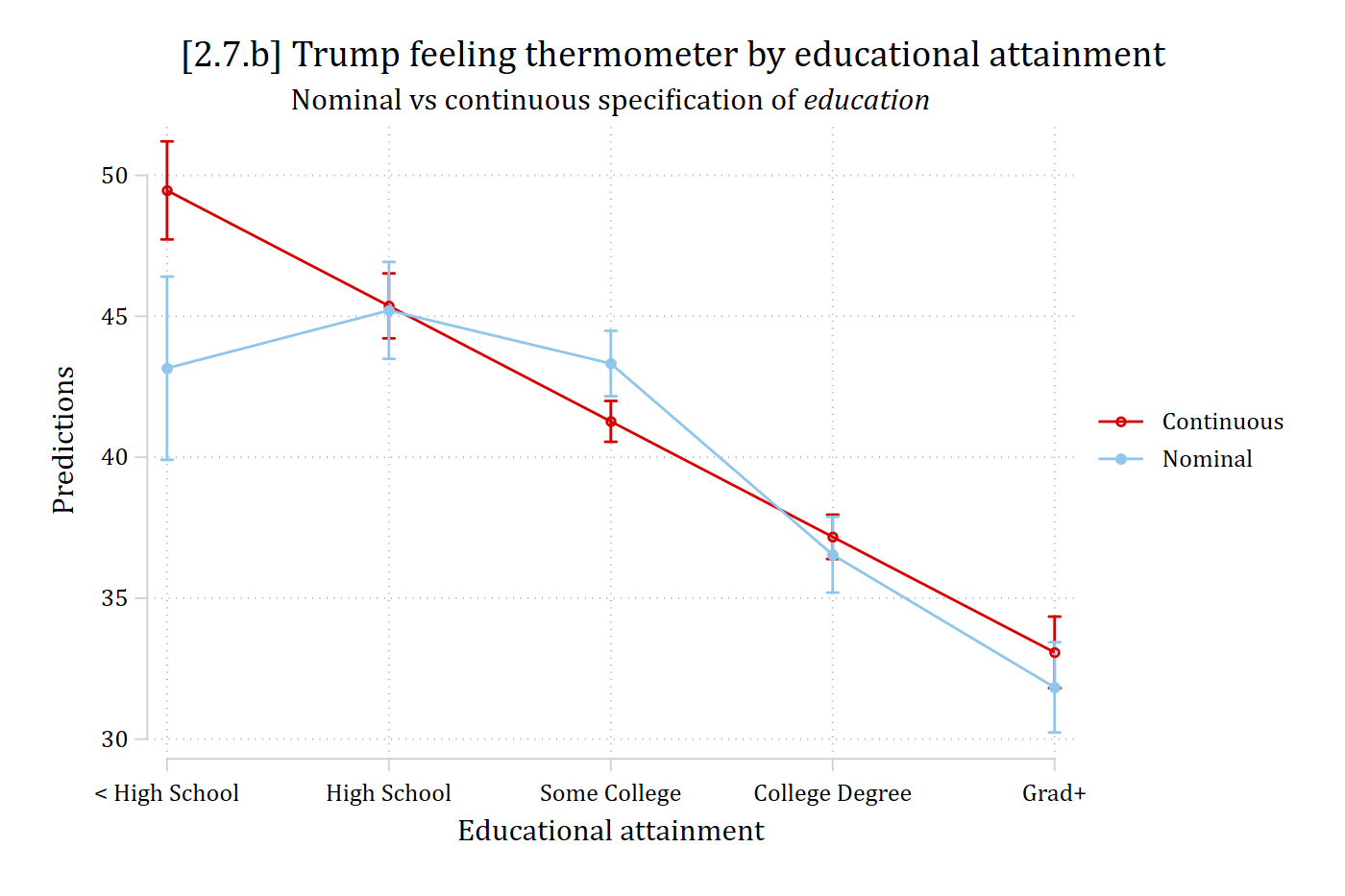
*These look quite different to me. I would not feel comfortable using the continuous specification and would instead use the nominal specification of educational attainment
Nominal independent variables
- The traditional approach for interpreting nominal IVs involves specifying an omitted reference category and interpreting the coefficients which represent contrasts between the omitted category and each included group
- An issue with this approach is you do not know how included categories compare to each other
- This approach also reifies the omitted category as the most important (Johfre and Freese 2021)
- You also do not have any sense of how large an effect the nominal IV has overall (only specific contrasts)
- An issue with this approach is you do not know how included categories compare to each other
- One partial solution is to plot predictions for all categories of the nominal IV
- There is no reference group in this approach
regress feel_trump c.relimport i.educ age hhincome i.woman ///
    i.lgb i.race4 i.wrongtrack
Source | SS df MS Number of obs = 7,155
-------------+---------------------------------- F(13, 7141) = 506.04
Model | 5562481.5 13 427883.192 Prob > F = 0.0000
Residual | 6038073.21 7,141 845.550093 R-squared = 0.4795
-------------+---------------------------------- Adj R-squared = 0.4786
Total | 11600554.7 7,154 1621.54804 Root MSE = 29.078
-------------------------------------------------------------------------------
feel_trump | Coefficient Std. err. t P>|t| [95% conf. interval]
--------------+----------------------------------------------------------------
relimport | -5.949 0.249 -23.879 0.000 -6.438 -5.461
|
educ |
2. High sc.. | 1.915 1.851 1.035 0.301 -1.713 5.543
3. Some po.. | 0.002 1.747 0.001 0.999 -3.422 3.426
4. Bachelo.. | -6.789 1.808 -3.755 0.000 -10.333 -3.244
5. Graduat.. | -11.486 1.880 -6.108 0.000 -15.173 -7.800
|
age | -0.051 0.021 -2.401 0.016 -0.093 -0.009
hhincome | -0.014 0.006 -2.501 0.012 -0.025 -0.003
|
woman |
Woman | -4.472 0.700 -6.392 0.000 -5.844 -3.101
|
lgb |
LGB | -10.331 1.409 -7.331 0.000 -13.093 -7.568
|
race4 |
Black | -24.256 1.274 -19.037 0.000 -26.754 -21.758
Hispanic | -11.116 1.230 -9.038 0.000 -13.527 -8.705
Other | -4.763 1.234 -3.861 0.000 -7.181 -2.345
|
wrongtrack |
Wrong track | -49.332 0.832 -59.312 0.000 -50.963 -47.702
_cons | 107.667 2.319 46.433 0.000 103.121 112.212
-------------------------------------------------------------------------------est store ftmod
margins race4Predictive margins Number of obs = 7,155
Model VCE: OLS
Expression: Linear prediction, predict()
------------------------------------------------------------------------------
| Delta-method
| Margin std. err. t P>|t| [95% conf. interval]
-------------+----------------------------------------------------------------
race4 |
White | 43.283 0.408 106.133 0.000 42.484 44.083
Black | 19.027 1.192 15.960 0.000 16.690 21.364
Hispanic | 32.167 1.150 27.979 0.000 29.913 34.421
Other | 38.521 1.161 33.171 0.000 36.244 40.797
------------------------------------------------------------------------------marginsplot, recast(scatter) ///
ylab(0(10)70) ytitle("Trump feeling thermometer") ///
title("[2.7.c] Feelings toward Trump based on race-ethnicity", size(medlar
ge))Variables that uniquely identify margins: race4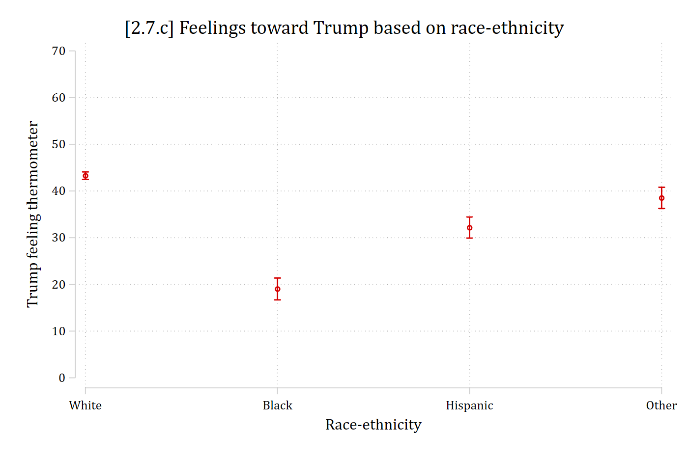
Examining all pairwise comparisons
- To obtain a significance test for all contrasts between all categories, you can conduct pairwise comparisons
mecompare race4, models(ftmod) pwcomparePredicting: Linear prediction
Marginal effects (N_ftmod=7155)
| ME # Estimate SE P>|z|
---------------------------------+---------------------------------------
race4 |
Black - White |
ftmod | 1 -24.256 1.274 0.000
Hispanic - White |
ftmod | 2 -11.116 1.230 0.000
Other - White |
ftmod | 3 -4.763 1.234 0.000
Hispanic - Black |
ftmod | 4 13.140 1.632 0.000
Other - Black |
ftmod | 5 19.494 1.664 0.000
Other - Hispanic |
ftmod | 6 6.354 1.627 0.000- Black adults feel less warmly toward Trump than do White adults
- …
- Hispanic adults feel more warmly toward Trump than do Black adults
- Etc.
Alternative interpretations of nominal IVs
- Some alternatives use different contrasts
- Mean contrasts compare a group to the overall sample mean
- Limitation is the group being compared is part of the overall sample
- Binary contrasts compare that group to all other groups (pooled)
- In Stata, use the binarycontrast command (Freese and Johfre 2022)
- In R, avg_predictions with hypothesis = ~ meanotherdev is similar, comparing group’s prediction to the mean across all other groups
- But, doesn’t account for differing group sizes
Quantifying holistic effects of nominal IVs
- An important issue with any pairwise comparison approach is the high chance of a Type I error (false positive)
- We will cover this more in the Testing section of the class
- Another set of alternatives examine the holistic effect of the IV
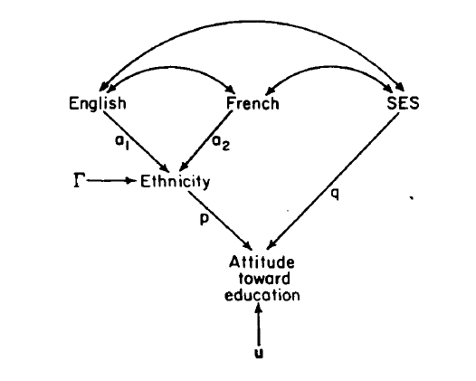
- The sheaf coefficient provides a single value for the overall effect of the nominal IV (Heise 1972)
- Key limitation is it has no clear/satisfying interpretation
- The sheaf coefficient provides a single value for the overall effect of the nominal IV (Heise 1972)
Marginal effect (ME) inequality statistics
- A new approach summarizes the average level of inequality patterned by the nominal IV using marginal effects (Mize and Han 2025)
- I.e., How different the predictions are across the nominal groupings, on average
- Define each pairwise comparison (category a vs. b) as a ME:
\[pairwise\ comparisons = ME = \eta\left( x_{k} = a,\mathbf{x}_{- k} = {\mathbf{x}_{- k}}^{*} \right) - \eta\left( x_{k} = b,\mathbf{x}_{- k} = {\mathbf{x}_{- k}}^{*} \right);\ for\ all\ b > a\]
- The unweighted ME inequality is simply the average of the (absolute values) of all pairwise comparisons
\[unweighted\ ME\ inequality \equiv |unweighted\ average\ ME\ inequality|\]
\[= \frac{Sum\ of\ all\ |pairwise\ comparisons\ of\ MEs|}{\#\ of\ comparisons}\]
\[= \frac{\sum_{a = 1}^{L}\sum_{b = 2;\ b > a}^{L}\left| \eta\left( x_{k} = a,\ \mathbf{x}_{- k} = {\mathbf{x}_{- k}}^{*} \right) - \eta\left( x_{k} = b,\mathbf{x}_{- k} = {\mathbf{x}_{- k}}^{*} \right) \right|}{\frac{L(L - 1)}{2}}\]
- Usually, the various groups of the nominal IV will differ in size, so should be given different weight in the ME inequality, proportional to their size
- Define weights
\[a\ vs\ b\ contrast\ weight = w_{a,b} = \frac{n_{a} + n_{b}}{N}\]
- The weighted ME inequality is then
\[ME\ inequality \equiv |weighted\ average\ ME\ inequality|\]
\[= \sum_{a = 1}^{L}\sum_{b = 2;\ b > a}^{L}\frac{w_{a,b}}{L - 1}*\left| \eta\left( x_{k} = a,\mathbf{x}_{- k} = {\mathbf{x}_{- k}}^{*} \right) - \eta\left( x_{k} = b,\mathbf{x}_{- k} = {\mathbf{x}_{- k}}^{*} \right) \right|\]
“…ME inequality can be described as the average difference in outcomes between observations in distinct groups.”
“Alternatively, ME inequality could be used to quantify a causal effect of a nominal or ordinal IV. In this case, ME inequality summarizes how outcomes would typically change if an observation switched from their current category to another category.” (Mize and Han 2025)
Calculating ME inequalities in Stata and R
- In Stata, use the meinequality command or the meinequality option on mecompare
- In R, use the meinq() function with avg_comparisons
meinequality race4, models(ftmod)ME Inequality Estimates (N = 7155)
| Estimate Std. err. z P>|z|
-------------------------+-----------------------------------------------
ME Inequality |
race4 | 13.303 0.699 19.026 0.000 On average, members of different racial-ethnic groups differ by about 13 points in their feelings towards Trump