Two continuous variables
Political views × survey year: Figures 15–17 of Mize (2019)
Interactions between two continuous variables are the hardest to present because there are an almost unlimited number of combinations of the two variables at which one could examine the effects. The article’s example is whether the growth in acceptance of same-sex relationships in the GSS between 1976 and 2016 has been broad-based or concentrated among people with particular political views. Political views are a standardized scale (0 = moderate, negative = liberal, positive = conservative); year is coded as years since 1976.
The model
use "https://tdmize.github.io/data/data/nli_gss", clear(GSS 1972-2016 | NLI NonLinear Interaction Effects | 2018-12-17)drop if missing(sameokB, year1976, conviewSS, age, white, male, income, married, college)(42,940 observations deleted)
. quietly logit sameokB c.year1976##c.year1976##c.conviewSS c.age i.white i.male ///
c.income i.married i.college, vce(robust)
estimates store samemodAverage effects of each variable
Before looking at the interaction, the average effect of a standard-deviation increase in each variable:
mecompare year1976 conviewSS, models(samemod) amount(sd) uncenteredPredicting: Pr(sameokB)
Marginal effects (N_samemod=19337)
| ME # Estimate Robust SE P>|z|
---------------------------------+---------------------------------------
year1976 + SD (uncentered) |
samemod | 1 0.150 0.003 0.000
---------------------------------+---------------------------------------
conviewSS + SD (uncentered) |
samemod | 2 -0.078 0.003 0.000More conservative individuals are less likely to view same-sex relationships as acceptable, and acceptance has risen over time.
Ideal types (Figure 15)
The first way to present the interaction is to pick “ideal types” on one variable – here one standard deviation below and above the mean of political views, labeled liberal and conservative – and plot the predictions across the other.
mecompare replaces the estimates in memory, so restore the model first.
estimates restore samemod(results samemod are active now)quietly margins, at(conviewSS=(-1 1) year1976=(0(2)40))
marginsplot, x(year1976) recastci(rline) ciopts(lpattern(dash)) ylabel(0(0.2)1) ///
plot1opts(lcolor(blue) mcolor(blue)) ci1opts(color(blue*.4)) ///
plot2opts(lcolor(red) mcolor(red)) ci2opts(color(red*.4)) ///
xlabel(0 "1976" 8 "1984" 16 "1992" 24 "2000" 32 "2008" 40 "2016") ///
xtitle("GSS survey year") ytitle("Pr(Same-sex relationships OK)") ///
legend(order(3 "Liberal" 4 "Conservative")) ///
title("Figure 15. Pr(same-sex OK) by political views and year")Variables that uniquely identify margins: conviewSS year1976graph export "fig/nli-sameok-predictions.png", replace width(1400)file fig/nli-sameok-predictions.png saved as PNG format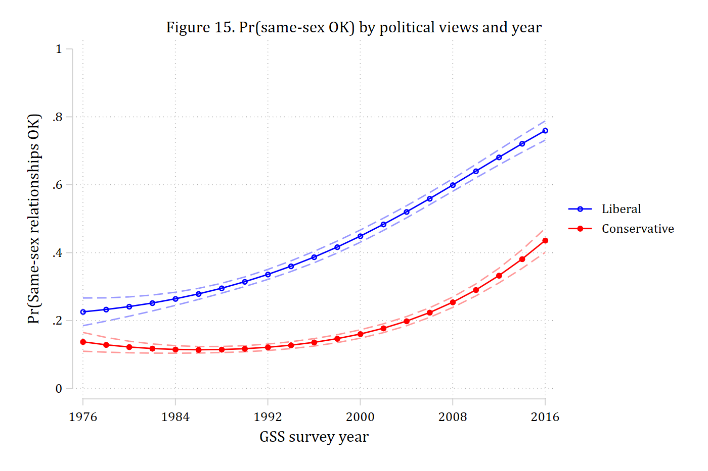
The effect of time at the two ideal types, and whether it differs, is the marginal effect of year with conviewSS held at each value:
mecompare year1976, models(samemod) covariates(conviewSS=(-1 1)) amount(rate)Predicting: Pr(sameokB)
Marginal effects (N_samemod=19337)
| ME # Estimate Robust SE P>|z|
---------------------------------+---------------------------------------
year1976(rate) |
conviewSS=-1 | 1 0.013 0.001 0.000
conviewSS=1 | 2 0.007 0.000 0.000metest 1 - 2 | estimate se pvalue
---------------------------------+--------------------------------
year1976_con~1 - year1976_con~1 | 0.006 0.001 0.000 One standard deviation above and below the mean are conventional ideal types, but a good default for any continuous moderator is its 10th, 50th, and 90th percentiles: a low, a typical, and a high value that are all in the range of the data. summarize, detail returns them, and they go straight into covariates(). The joint test is the test of interaction on this side, and any pair can be tested as before:
quietly summarize conviewSS, detail
local p10 : display %5.2f r(p10)
local p50 : display %5.2f r(p50)
local p90 : display %5.2f r(p90)
mecompare year1976, models(samemod) covariates(conviewSS=(`p10' `p50' `p90')) amount(rate)
Predicting: Pr(sameokB)
Marginal effects (N_samemod=19337)
| ME # Estimate Robust SE P>|z|
---------------------------------+---------------------------------------
year1976(rate) |
conviewSS=-.8 | 1 0.012 0.000 0.000
conviewSS=-.07 | 2 0.010 0.000 0.000
conviewSS=.87 | 3 0.007 0.000 0.000metest 1 = 2 = 3Tests of equality
| chi2 df pvalue
---------------------------------+--------------------------------
year19~8 = year1~07 = year1~87 | 75.993 2.000 0.000 metest 3 - 1 | estimate se pvalue
---------------------------------+--------------------------------
year1976_co~87 - year1976_con~8 | -0.005 0.001 0.000 The effect of political views across years (Figure 16)
The second way to present the interaction is to plot the marginal effect of one variable across the range of the other. First the test the article reports: the effect of political views in 1976 versus 2016, the instantaneous effect (amount(rate)) with year held at 0 and at 40.
mecompare conviewSS, models(samemod) covariates(year1976=(0 40)) amount(rate)Predicting: Pr(sameokB)
Marginal effects (N_samemod=19337)
| ME # Estimate Robust SE P>|z|
---------------------------------+---------------------------------------
conviewSS(rate) |
year1976=0 | 1 -0.044 0.016 0.005
year1976=40 | 2 -0.159 0.013 0.000metest 2 - 1 | estimate se pvalue
---------------------------------+--------------------------------
conviewSS_y~40 - conviewSS_ye~0 | -0.115 0.016 0.000 Political views matter more in 2016 than in 1976: the effect is negative in both years and significantly larger in magnitude in the later one. The same test at the 10th, 50th, and 90th percentiles of survey year:
quietly summarize year1976, detail
mecompare conviewSS, models(samemod) covariates(year1976=(`r(p10)' `r(p50)' `r(p90)')) amount(rate
)
Predicting: Pr(sameokB)
Marginal effects (N_samemod=19337)
| ME # Estimate Robust SE P>|z|
---------------------------------+---------------------------------------
conviewSS(rate) |
year1976=4 | 1 -0.059 0.010 0.000
year1976=18 | 2 -0.115 0.005 0.000
year1976=36 | 3 -0.170 0.009 0.000metest 1 = 2 = 3Tests of equality
| chi2 df pvalue
---------------------------------+--------------------------------
convie~4 = convi~18 = convi~36 | 72.929 2.000 0.000 metest 3 - 1 | estimate se pvalue
---------------------------------+--------------------------------
conviewSS_y~36 - conviewSS_ye~4 | -0.111 0.013 0.000 Across all years:
mecompare conviewSS, models(samemod) covariates(year1976=(0(4)40)) amount(rate) store(pv)Predicting: Pr(sameokB)
Marginal effects (N_samemod=19337)
| ME # Estimate Robust SE P>|z|
---------------------------------+---------------------------------------
conviewSS(rate) |
year1976=0 | 1 -0.044 0.016 0.005
year1976=4 | 2 -0.059 0.010 0.000
year1976=8 | 3 -0.074 0.007 0.000
year1976=12 | 4 -0.090 0.005 0.000
year1976=16 | 5 -0.106 0.005 0.000
year1976=20 | 6 -0.123 0.006 0.000
year1976=24 | 7 -0.141 0.006 0.000
year1976=28 | 8 -0.157 0.006 0.000
year1976=32 | 9 -0.168 0.007 0.000
year1976=36 | 10 -0.170 0.009 0.000
year1976=40 | 11 -0.159 0.013 0.000
. coefplot pv_samemod, vertical recast(connected) color(black) ///
ciopts(recast(rline) lpattern(dash) color(gs12)) yline(0) ///
rename("^.*=0$" = 1976 "^.*=4$" = 1980 "^.*=8$" = 1984 ///
"^.*=12$" = 1988 "^.*=16$" = 1992 "^.*=20$" = 1996 ///
"^.*=24$" = 2000 "^.*=28$" = 2004 "^.*=32$" = 2008 ///
"^.*=36$" = 2012 "^.*=40$" = 2016, regex) ///
ylabel(-0.25(0.05)0.05) xtitle("GSS survey year") ///
ytitle("AME of conservative political views") ///
title("Figure 16. AME of political views by survey year") ///
note("Negative effects indicate conservatives are less supportive of same-sex relationships")
graph export "fig/nli-sameok-views-by-year.png", replace width(1400)file fig/nli-sameok-views-by-year.png saved as PNG format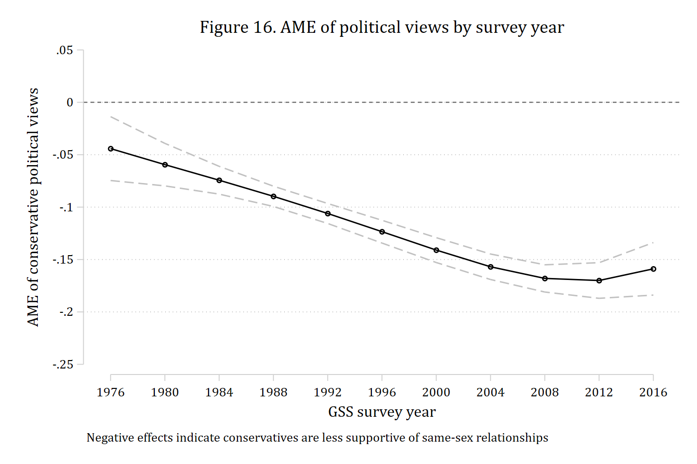
The effect of time across political views (Figure 17)
The other side: how much acceptance has changed over time for people with different views. The article reports a two-year change (the survey interval) for liberals and conservatives:
mecompare year1976, models(samemod) covariates(conviewSS=(-1 1)) amount(2) uncenteredPredicting: Pr(sameokB)
Marginal effects (N_samemod=19337)
| ME # Estimate Robust SE P>|z|
---------------------------------+---------------------------------------
year1976 + 2 (uncentered) |
conviewSS=-1 | 1 0.026 0.001 0.000
conviewSS=1 | 2 0.015 0.001 0.000metest 1 - 2 | estimate se pvalue
---------------------------------+--------------------------------
year1976_con~1 - year1976_con~1 | 0.011 0.002 0.000 Everyone has become more accepting, liberals significantly more so than conservatives per two-year interval. Across the range of political views, from two standard deviations below the mean to two above, in steps of one half:
mecompare year1976, models(samemod) covariates(conviewSS=(-2(0.5)2)) amount(2) uncentered store(tm
)
Predicting: Pr(sameokB)
Marginal effects (N_samemod=19337)
| ME # Estimate Robust SE P>|z|
---------------------------------+---------------------------------------
year1976 + 2 (uncentered) |
conviewSS=-2 | 1 0.029 0.002 0.000
conviewSS=-1.5 | 2 0.028 0.002 0.000
conviewSS=-1 | 3 0.026 0.001 0.000
conviewSS=-.5 | 4 0.024 0.001 0.000
conviewSS=0 | 5 0.021 0.001 0.000
conviewSS=.5 | 6 0.018 0.001 0.000
conviewSS=1 | 7 0.015 0.001 0.000
conviewSS=1.5 | 8 0.012 0.001 0.000
conviewSS=2 | 9 0.009 0.001 0.000
. coefplot tm_samemod, vertical recast(connected) color(black) ///
ciopts(recast(rline) lpattern(dash) color(gs12)) yline(0) ///
rename("^.*=-2$" = "Very liberal" "^.*=-1$" = "Liberal" "^.*=0$" = "Moderate" ///
"^.*=1$" = "Conservative" "^.*=2$" = "Very conservative", regex) ///
coeflabels(*5 = " ") ///
xtitle("") ytitle("Effect of two years on Pr(Same-sex relationships OK)") ///
title("Figure 17. AME of time by political views") ///
note("Positive effects: the group has become more supportive over time")
graph export "fig/nli-sameok-time-by-views.png", replace width(1400)file fig/nli-sameok-time-by-views.png saved as PNG format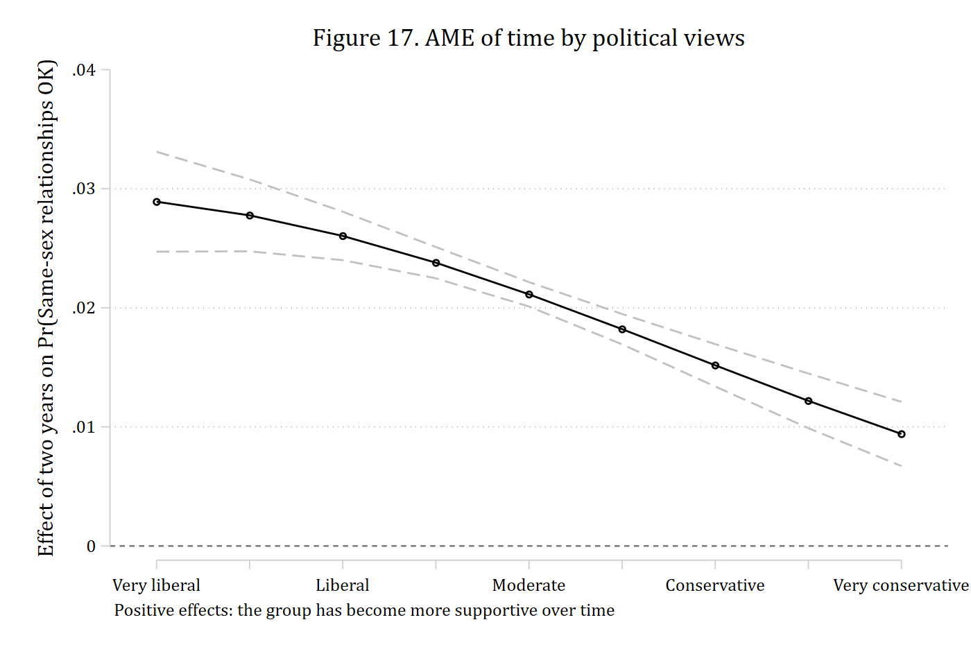
Predictions over both variables (Figure 18)
The article’s final figure shows the predictions at every combination of the two variables as a contour plot, made with margins and twoway contour. margins, saving() saves the predictions on a grid of both variables (nose skips the standard errors); the saved dataset holds the predictions in _margin and the grid values in _at1 and _at2.
estimates restore samemod(results samemod are active now)tempfile preds
quietly margins, at(conviewSS=(-2(.1)2) year1976=(0(2)40)) nose saving(`preds', replace). use `preds', clear(Created by command margins; also see char list)rename _at1 year1976
rename _at2 conviewSS
rename _margin pr_sameok. twoway (contour pr_sameok conviewSS year1976, ccuts(0(0.05)1) ///
scolor(red) ecolor(purple) crule(hue)), ///
xlabel(0 "1976" 8 "1984" 16 "1992" 24 "2000" 32 "2008" 40 "2016") ///
ylabel(-2 "Very liberal" -1 "Liberal" 0 "Moderate" 1 "Conservative" 2 "Very conservative") ///
zlabel(0(0.1)1) ztitle("Pr(Same-sex relationships OK)") ///
xtitle("") ytitle("") xsize(7) ysize(4) ///
title("Figure 18. Pr(same-sex OK) across political views and year")
graph export "fig/nli-sameok-contour.png", replace width(1400)file fig/nli-sameok-contour.png saved as PNG format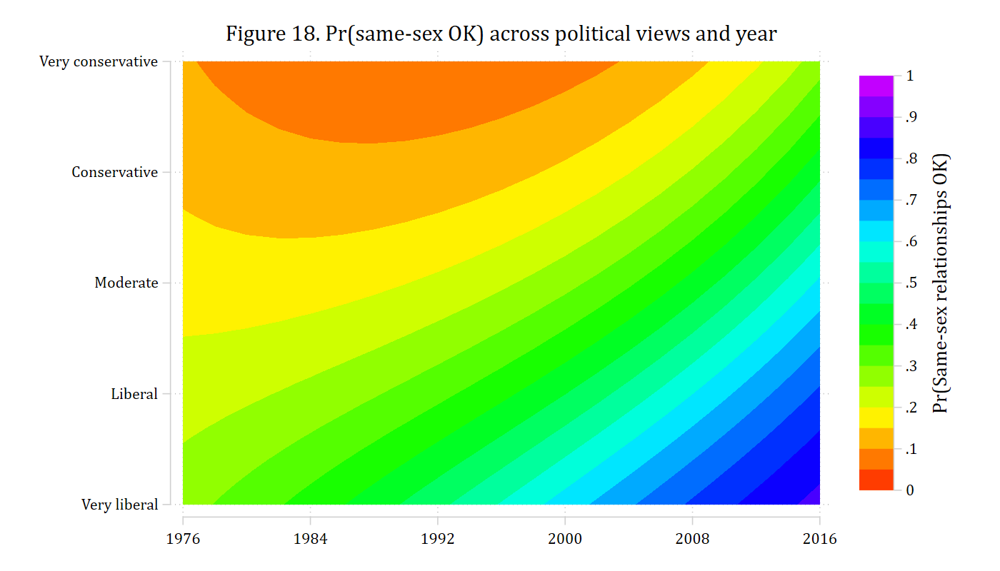
The replication files at trentonmize.com/research also include a grayscale version (scolor(black) ecolor(gs16) crule(linear)).