Plotting and tabulating results
store() with coefplot and esttab
The store(stub) option saves the marginal effects as stored estimates – one for each model and one for the differences – so that coefplot and esttab (Jann) can plot and table them. Install both once with ssc install coefplot and ssc install estout.
Fit, store, compare
sysuse nlsw88, clear(NLSW, 1988 extract)drop if missing(union, married, age, race, hours, collgrad, ttl_exp, grade, wage)(371 observations deleted)
. quietly logit union i.married age i.race hours i.collgrad ttl_exp, vce(robust)
estimates store m1
quietly logit union i.married age i.race hours i.collgrad ttl_exp grade wage, vce(robust)
estimates store m2. mecompare i.married age i.race hours i.collgrad ttl_exp, models(m1 m2) store(mec)Predicting: Pr(union)
Marginal effects and cross-model differences (N_m1=1875) (N_m2=1875)
| ME # Estimate Robust SE P>|z|
---------------------------------+---------------------------------------
married |
Married - Single |
m1 | 1 -0.025 0.022 0.238
m2 | 2 -0.019 0.021 0.367
Difference | 3 -0.006 0.003 0.036
---------------------------------+---------------------------------------
age + 1 (centered) |
m1 | 4 0.002 0.003 0.547
m2 | 5 0.003 0.003 0.363
Difference | 6 -0.001 0.001 0.049
---------------------------------+---------------------------------------
race |
Black - White |
m1 | 7 0.078 0.024 0.001
m2 | 8 0.094 0.024 0.000
Difference | 9 -0.016 0.005 0.001
Other - White |
m1 | 10 0.101 0.098 0.303
m2 | 11 0.089 0.101 0.378
Difference | 12 0.012 0.015 0.432
---------------------------------+---------------------------------------
hours + 1 (centered) |
m1 | 13 0.002 0.001 0.132
m2 | 14 0.002 0.001 0.153
Difference | 15 0.000 0.000 0.724
---------------------------------+---------------------------------------
collgrad |
College gra - Not colleg |
m1 | 16 0.099 0.025 0.000
m2 | 17 0.043 0.039 0.264
Difference | 18 0.056 0.032 0.083
---------------------------------+---------------------------------------
ttl exp + 1 (centered) |
m1 | 19 0.003 0.002 0.223
m2 | 20 -0.001 0.002 0.558
Difference | 21 0.004 0.001 0.000This saved mec_m1, mec_m2, and mec_diff.
Plotting both models’ marginal effects
coefplot mec_m1 mec_m2, xline(0) xtitle("Average marginal effect on Pr(union)")
graph export "fig/plotting-both-models.png", replace width(1400)
file fig/plotting-both-models.png saved as PNG format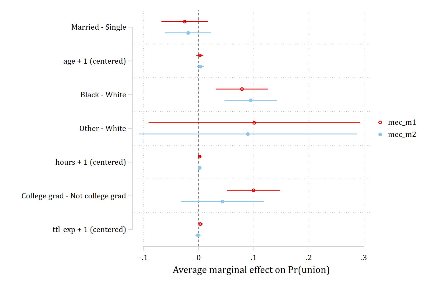
Plotting the cross-model differences
coefplot mec_diff, xline(0) xtitle("Difference in marginal effect (model 1 - model 2)")
graph export "fig/plotting-differences.png", replace width(1400)
file fig/plotting-differences.png saved as PNG format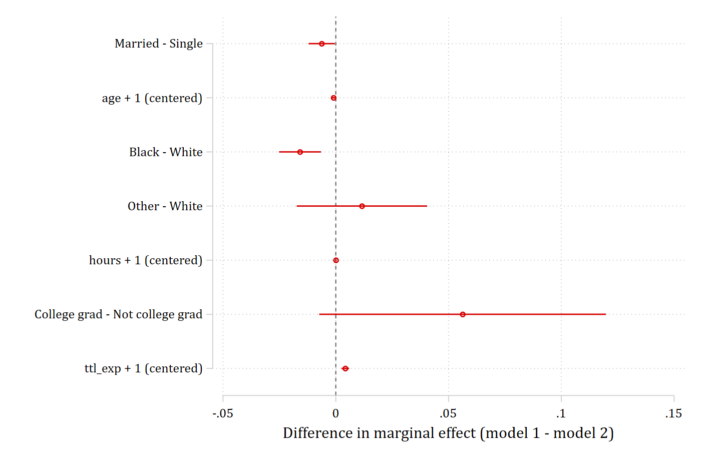
A three-column table
esttab mec_m1 mec_m2 mec_diff, se mtitles("Model 1" "Model 2" "Difference") nonumbers------------------------------------------------------------
Model 1 Model 2 Difference
------------------------------------------------------------
Married - ~e -0.0254 -0.0192 -0.00624*
(0.0215) (0.0213) (0.00298)
age + 1 (c~) 0.00198 0.00297 -0.000994*
(0.00329) (0.00327) (0.000506)
Black - Wh~e 0.0783** 0.0942*** -0.0159***
(0.0239) (0.0243) (0.00473)
Other - Wh~e 0.101 0.0890 0.0116
(0.0977) (0.101) (0.0148)
hours + 1 ~) 0.00156 0.00150 0.0000601
(0.00104) (0.00105) (0.000170)
College gr~d 0.0993*** 0.0430 0.0562
(0.0245) (0.0385) (0.0324)
ttl_exp + ~) 0.00279 -0.00143 0.00421***
(0.00229) (0.00244) (0.000867)
------------------------------------------------------------
N 1875 1875 1875
------------------------------------------------------------
Standard errors in parentheses
* p<0.05, ** p<0.01, *** p<0.001esttab takes all of its usual options (b(3), star, label, using file.rtf, …), so the same line writes a publication table.
One model
With one model store() saves a single estimate, stub followed by the model’s name (me1_m1 here):
mecompare i.married age i.race hours i.collgrad ttl_exp, models(m1) store(me1)Predicting: Pr(union)
Marginal effects (N_m1=1875)
| ME # Estimate Robust SE P>|z|
---------------------------------+---------------------------------------
married |
Married - Single |
m1 | 1 -0.025 0.022 0.238
---------------------------------+---------------------------------------
age + 1 (centered) |
m1 | 2 0.002 0.003 0.547
---------------------------------+---------------------------------------
race |
Black - White |
m1 | 3 0.078 0.024 0.001
Other - White |
m1 | 4 0.101 0.098 0.303
---------------------------------+---------------------------------------
hours + 1 (centered) |
m1 | 5 0.002 0.001 0.132
---------------------------------+---------------------------------------
collgrad |
College gra - Not colleg |
m1 | 6 0.099 0.025 0.000
---------------------------------+---------------------------------------
ttl exp + 1 (centered) |
m1 | 7 0.003 0.002 0.223coefplot me1_m1, xline(0) xtitle("Average marginal effect on Pr(union)")
graph export "fig/plotting-one-model.png", replace width(1400)file fig/plotting-one-model.png saved as PNG format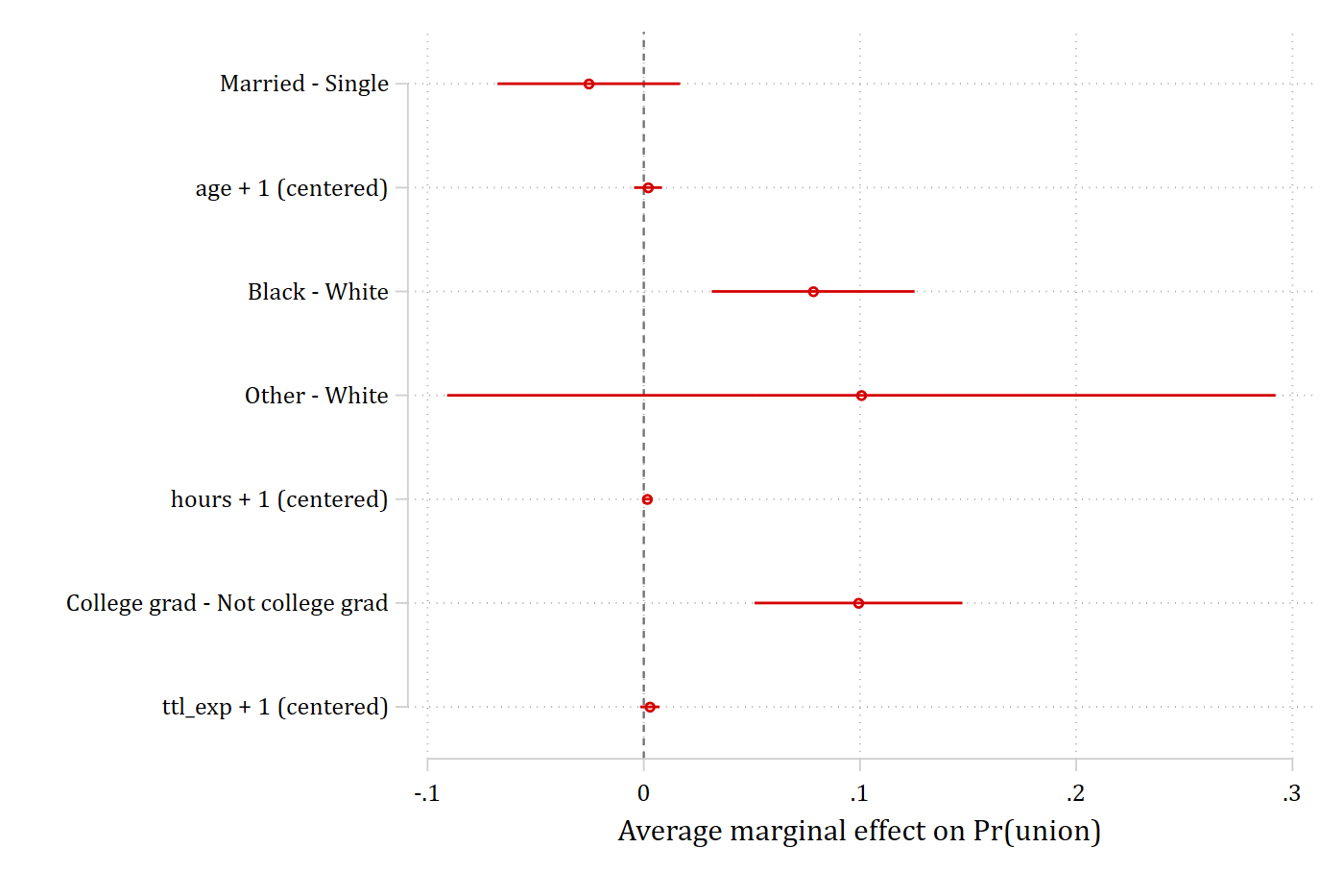
Effects across levels of a moderator
With by(), over(), or a covariates() value list, each stored estimate carries one coefficient per level, so the plot shows how an effect changes across the moderator. The coefficients are named with the table’s labels, e.g. age + 1 (centered), hours=20; rename() with a regular expression keeps the value after the =.
mecompare age, models(m1 m2) covariates(hours=(20 30 40 50 60)) store(byhrs)Predicting: Pr(union)
Marginal effects and cross-model differences (N_m1=1875) (N_m2=1875)
| ME # Estimate Robust SE P>|z|
---------------------------------+---------------------------------------
age + 1 (centered) |
m1 hours=20 | 1 0.002 0.003 0.547
m1 hours=30 | 2 0.002 0.003 0.547
m1 hours=40 | 3 0.002 0.003 0.547
m1 hours=50 | 4 0.002 0.003 0.548
m1 hours=60 | 5 0.002 0.004 0.548
m2 hours=20 | 6 0.003 0.003 0.362
m2 hours=30 | 7 0.003 0.003 0.362
m2 hours=40 | 8 0.003 0.003 0.363
m2 hours=50 | 9 0.003 0.003 0.364
m2 hours=60 | 10 0.003 0.004 0.364
Difference hours=20 | 11 -0.001 0.000 0.051
Difference hours=30 | 12 -0.001 0.000 0.050
Difference hours=40 | 13 -0.001 0.001 0.050
Difference hours=50 | 14 -0.001 0.001 0.050
Difference hours=60 | 15 -0.001 0.001 0.052coefplot (byhrs_m1, label("Model 1")) (byhrs_m2, label("Model 2")), vertical yline(0) ///
rename("^.*=(.*)$" = \1, regex) ///
xtitle("Hours worked per week") ytitle("Marginal effect of age on Pr(union)")
graph export "fig/plotting-moderator.png", replace width(1400)file fig/plotting-moderator.png saved as PNG format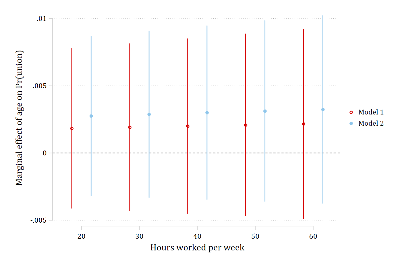
The interactions pages use this pattern to reproduce the marginal-effect figures of Mize (2019).