Options
Every option of balanceplot with group(), with an example of each
balanceplot varlist [if] [in], group(varname) [options]The examples use the nlsw88 data that ships with Stata and compare union and nonunion workers. The contreat() and tebalance forms of the command, and the table and store() options, have their own pages.
sysuse nlsw88, clear(NLSW, 1988 extract)balanceplot wage age i.married i.race tenure, group(union)NOTE: 10 observations were excluded due to missing data on
at least one covariate, group(), or outcome() variable.
Base category = 0_Nonunion
Base selected by the 0/1 two-group default.
N used in balance calculations
- N for union = 0_Nonunion: 1408
- N for union = 1_Union: 460graph export "fig/options-default.png", replace width(1400)file fig/options-default.png saved as PNG format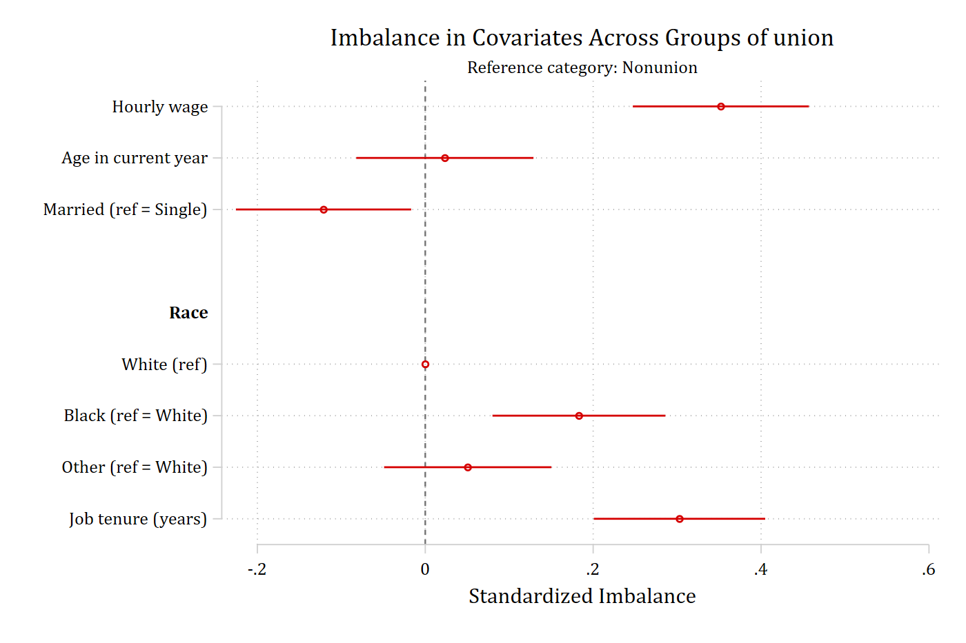
Which group is the base: base()
Each nonbase group is compared with the base. For a binary grouping variable the lowest category is the base by default; for three or more categories, the largest complete-case category. base() picks another.
balanceplot wage age i.married i.race tenure, group(union) base(1)NOTE: 10 observations were excluded due to missing data on
at least one covariate, group(), or outcome() variable.
Base category = 1_Union
N used in balance calculations
- N for union = 0_Nonunion: 1408
- N for union = 1_Union: 460graph export "fig/options-base.png", replace width(1400)file fig/options-base.png saved as PNG format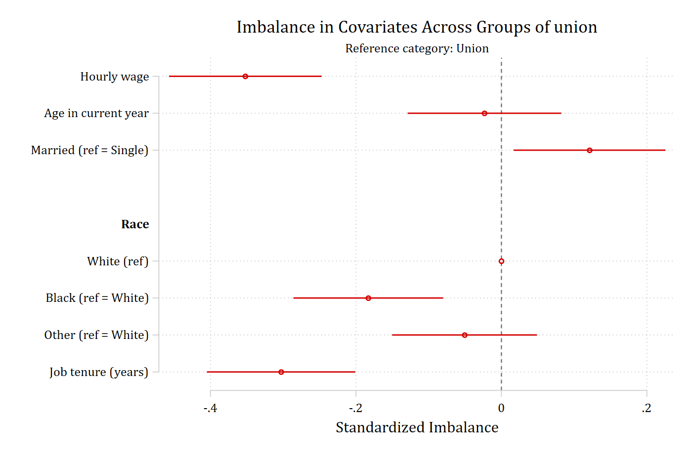
More than two groups
A grouping variable with several categories produces one comparison per nonbase category, each in its own color. leg1() and leg2() relabel the first two comparisons in the legend.
balanceplot wage age i.married tenure, group(race)NOTE: 15 observations were excluded due to missing data on
at least one covariate, group(), or outcome() variable.
Base category = 1_White
Base selected as the largest complete-case group.
N used in balance calculations
- N for race = 1_White: 1627
- N for race = 2_Black: 578
- N for race = 3_Other: 26graph export "fig/options-groups.png", replace width(1400)file fig/options-groups.png saved as PNG format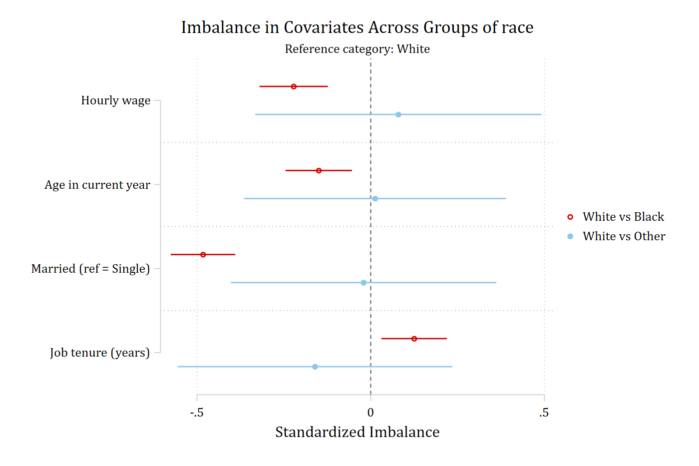
balanceplot wage age i.married tenure, group(race) ///
    leg1("Black relative to White") leg2("Other relative to White")
NOTE: 15 observations were excluded due to missing data on
at least one covariate, group(), or outcome() variable.
Base category = 1_White
Base selected as the largest complete-case group.
N used in balance calculations
- N for race = 1_White: 1627
- N for race = 2_Black: 578
- N for race = 3_Other: 26graph export "fig/options-legend.png", replace width(1400)file fig/options-legend.png saved as PNG format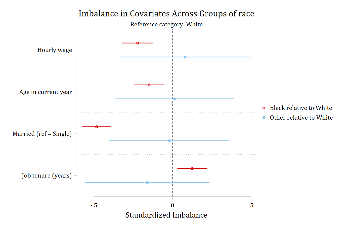
Cohen’s h for binary and nominal covariates: cohensh
By default every covariate is reported as a standardized mean difference. cohensh switches the binary and nominal covariates to Cohen’s h; the continuous covariates are unchanged. cohensH is a synonym.
balanceplot wage age i.married i.race tenure, group(union) cohenshNOTE: 10 observations were excluded due to missing data on
at least one covariate, group(), or outcome() variable.
Base category = 0_Nonunion
Base selected by the 0/1 two-group default.
N used in balance calculations
- N for union = 0_Nonunion: 1408
- N for union = 1_Union: 460graph export "fig/options-cohensh.png", replace width(1400)file fig/options-cohensh.png saved as PNG format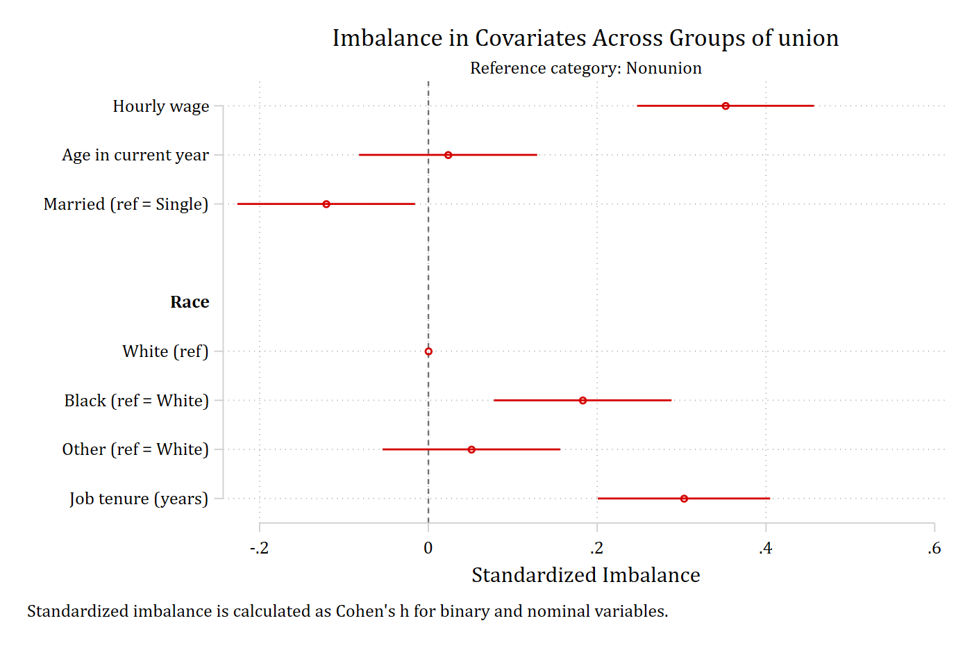
The estimation sample: outcome()
outcome() names a variable that is used only for listwise deletion, so that the balance sample matches a model that will include it. The variable is not plotted.
balanceplot age i.married i.race tenure, group(union) outcome(wage)NOTE: 10 observations were excluded due to missing data on
at least one covariate, group(), or outcome() variable.
Base category = 0_Nonunion
Base selected by the 0/1 two-group default.
N used in balance calculations
- N for union = 0_Nonunion: 1408
- N for union = 1_Union: 460
Complete-case sample additionally restricted by outcome(wage).Confidence intervals: level(), noci, and fadens
level() sets the confidence level (the default is 95) and noci drops the intervals from the graph; they remain in the returned matrices and in the tables. fadens keeps the intervals but fades the estimates that are not significant.
balanceplot wage age i.married i.race tenure, group(union) level(90)NOTE: 10 observations were excluded due to missing data on
at least one covariate, group(), or outcome() variable.
Base category = 0_Nonunion
Base selected by the 0/1 two-group default.
N used in balance calculations
- N for union = 0_Nonunion: 1408
- N for union = 1_Union: 460graph export "fig/options-level.png", replace width(1400)file fig/options-level.png saved as PNG format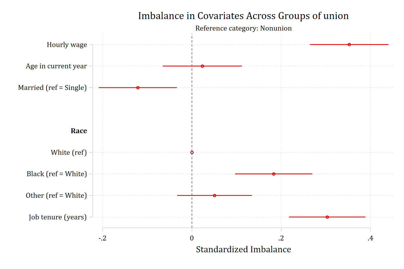
balanceplot wage age i.married i.race tenure, group(union) nociNOTE: 10 observations were excluded due to missing data on
at least one covariate, group(), or outcome() variable.
Base category = 0_Nonunion
Base selected by the 0/1 two-group default.
N used in balance calculations
- N for union = 0_Nonunion: 1408
- N for union = 1_Union: 460graph export "fig/options-noci.png", replace width(1400)file fig/options-noci.png saved as PNG format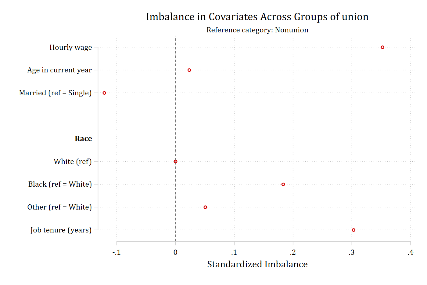
balanceplot wage age i.married i.race tenure, group(union) fadensNOTE: 10 observations were excluded due to missing data on
at least one covariate, group(), or outcome() variable.
Base category = 0_Nonunion
Base selected by the 0/1 two-group default.
N used in balance calculations
- N for union = 0_Nonunion: 1408
- N for union = 1_Union: 460graph export "fig/options-fadens.png", replace width(1400)file fig/options-fadens.png saved as PNG format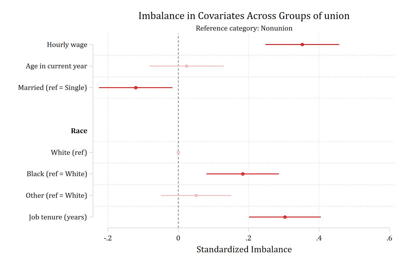
Reference lines: threshold()
threshold(#) adds dashed reference lines at -# and #, a common convention being 0.1.
balanceplot wage age i.married i.race tenure, group(union) threshold(.1)NOTE: 10 observations were excluded due to missing data on
at least one covariate, group(), or outcome() variable.
Base category = 0_Nonunion
Base selected by the 0/1 two-group default.
N used in balance calculations
- N for union = 0_Nonunion: 1408
- N for union = 1_Union: 460graph export "fig/options-threshold.png", replace width(1400)file fig/options-threshold.png saved as PNG format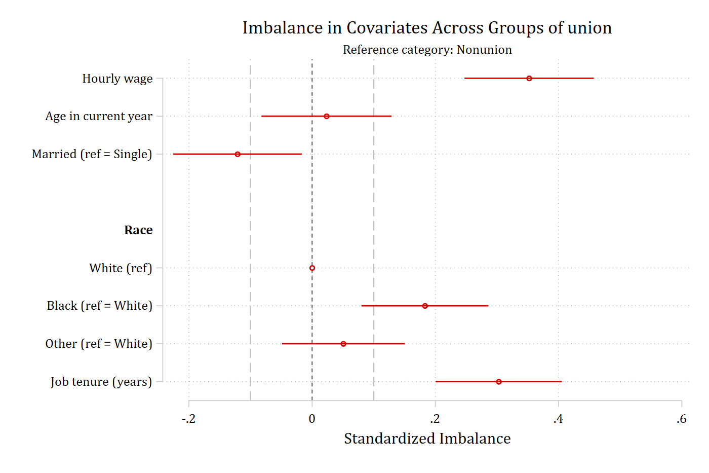
Ordering and sign: sort and absolute
By default covariates appear in the order of varlist, with the categories of a nominal covariate kept together under a heading. sort orders them from the most negative to the most positive imbalance (and drops the headings). absolute plots the magnitude of each imbalance; combined with sort, the covariates run from the most to the least balanced. abs is the shortest abbreviation.
balanceplot wage age i.married i.race tenure, group(union) sortNOTE: 10 observations were excluded due to missing data on
at least one covariate, group(), or outcome() variable.
Base category = 0_Nonunion
Base selected by the 0/1 two-group default.
N used in balance calculations
- N for union = 0_Nonunion: 1408
- N for union = 1_Union: 460graph export "fig/options-sort.png", replace width(1400)file fig/options-sort.png saved as PNG format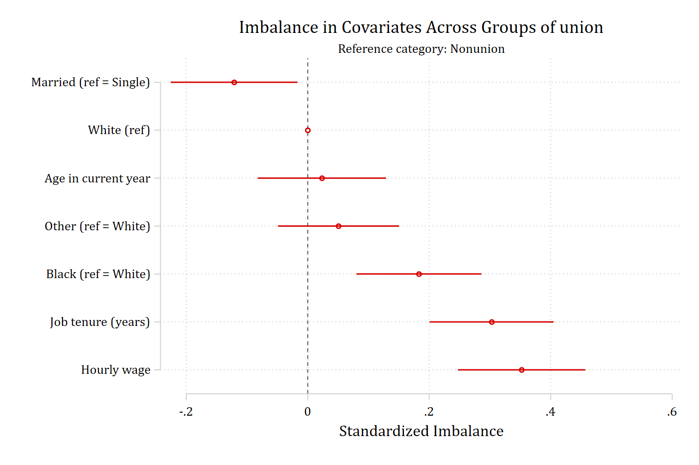
balanceplot wage age i.married i.race tenure, group(union) absolute sort threshold(.1)NOTE: 10 observations were excluded due to missing data on
at least one covariate, group(), or outcome() variable.
Base category = 0_Nonunion
Base selected by the 0/1 two-group default.
N used in balance calculations
- N for union = 0_Nonunion: 1408
- N for union = 1_Union: 460graph export "fig/options-absolute.png", replace width(1400)file fig/options-absolute.png saved as PNG format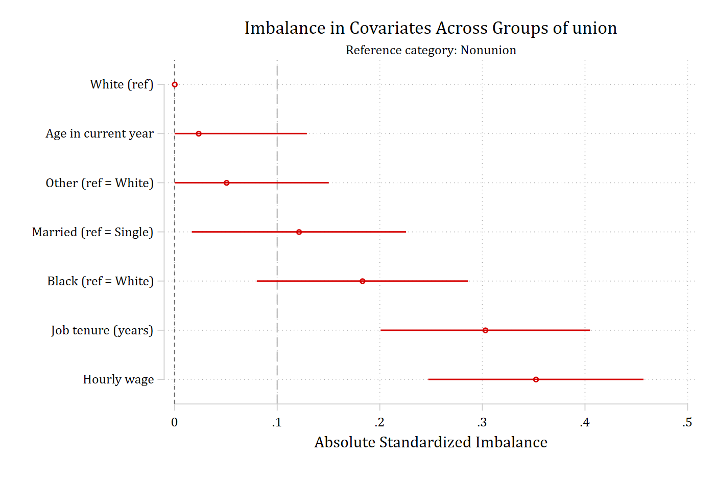
The graph itself: graphop(), leftmargin(), and plotcommand
balanceplot draws with coefplot, and graphop() passes any options through to it. leftmargin(#) widens the left margin of the graph region for long labels. plotcommand prints the coefplot command that produced the graph, which is the starting point for a fully customized version.
balanceplot wage age i.married i.race tenure, group(union) ///
    graphop(title("Union membership") xlabel(-.4(.2).6) note("NLSW 1988"))
NOTE: 10 observations were excluded due to missing data on
at least one covariate, group(), or outcome() variable.
Base category = 0_Nonunion
Base selected by the 0/1 two-group default.
N used in balance calculations
- N for union = 0_Nonunion: 1408
- N for union = 1_Union: 460graph export "fig/options-graphop.png", replace width(1400)file fig/options-graphop.png saved as PNG format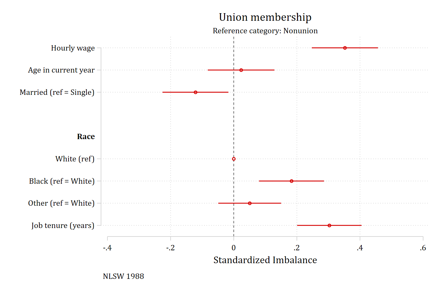
balanceplot wage age i.married i.race tenure, group(union) plotcommandNOTE: 10 observations were excluded due to missing data on
at least one covariate, group(), or outcome() variable.
Base category = 0_Nonunion
Base selected by the 0/1 two-group default.
N used in balance calculations
- N for union = 0_Nonunion: 1408
- N for union = 1_Union: 460
Matrices used for the plot: bias_0_1
Basic plot command:
coefplot (matrix(bias_0_1[,4]), ci((bias_0_1[,6] bias_0_1[,7])) label(`"Nonunion vs Union"'))The command is also returned in r(plotcommand).
Tables and stored results
table, tablefull, their formatting options decimals(), width(), and labwidth(), the store() option for esttab, and the returned matrices are on the Tables and stored results page. matchweight(), which adds the balance after matching to the same graph, is on the Matching and teffects page.