Nonlinear effects in a linear model
Age, age², and gender: Table 2 and Figures 1–2 of Mize (2019)
Even linear regression models often produce nonlinear effects, e.g. when the model has a polynomial specification such as a squared term. In the case of nonlinearities, questions like “does the effect of age differ for men and women?” have no single answer: it depends on where in the range of age you ask. The article’s first example regresses hourly wages on age, age², gender, and their products, using employed respondents from the pooled GSS.
The model
use "https://tdmize.github.io/data/data/nli_gss", clear(GSS 1972-2016 | NLI NonLinear Interaction Effects | 2018-12-17)drop if missing(wages, age, woman, parent, year, race, college, parttime, employed)(31,346 observations deleted)keep if employed == 1(0 observations deleted)
. quietly regress wages c.age##c.age##i.woman i.parent c.year i.race i.college i.parttime, vce(robus
t)
estimates store regwagesStart with the predictions (Figure 1)
The article recommends plotting the predictions first, with margins and marginsplot, and letting the plot guide the tests.
quietly margins woman, at(age=(18(2)72))
marginsplot, recastci(rline) ciopts(lpattern(dash) color(*.4)) ///
    plotopts(lwidth(medthick) msymbol(none)) ///
    xlabel(20(10)70) ylabel(0(5)25) xtitle("Age in years") ytitle("Hourly wages") ///
    title("Figure 1. Predicted wages by age and gender")
Variables that uniquely identify margins: age womangraph export "fig/nli-wages-predictions.png", replace width(1400)file fig/nli-wages-predictions.png saved as PNG format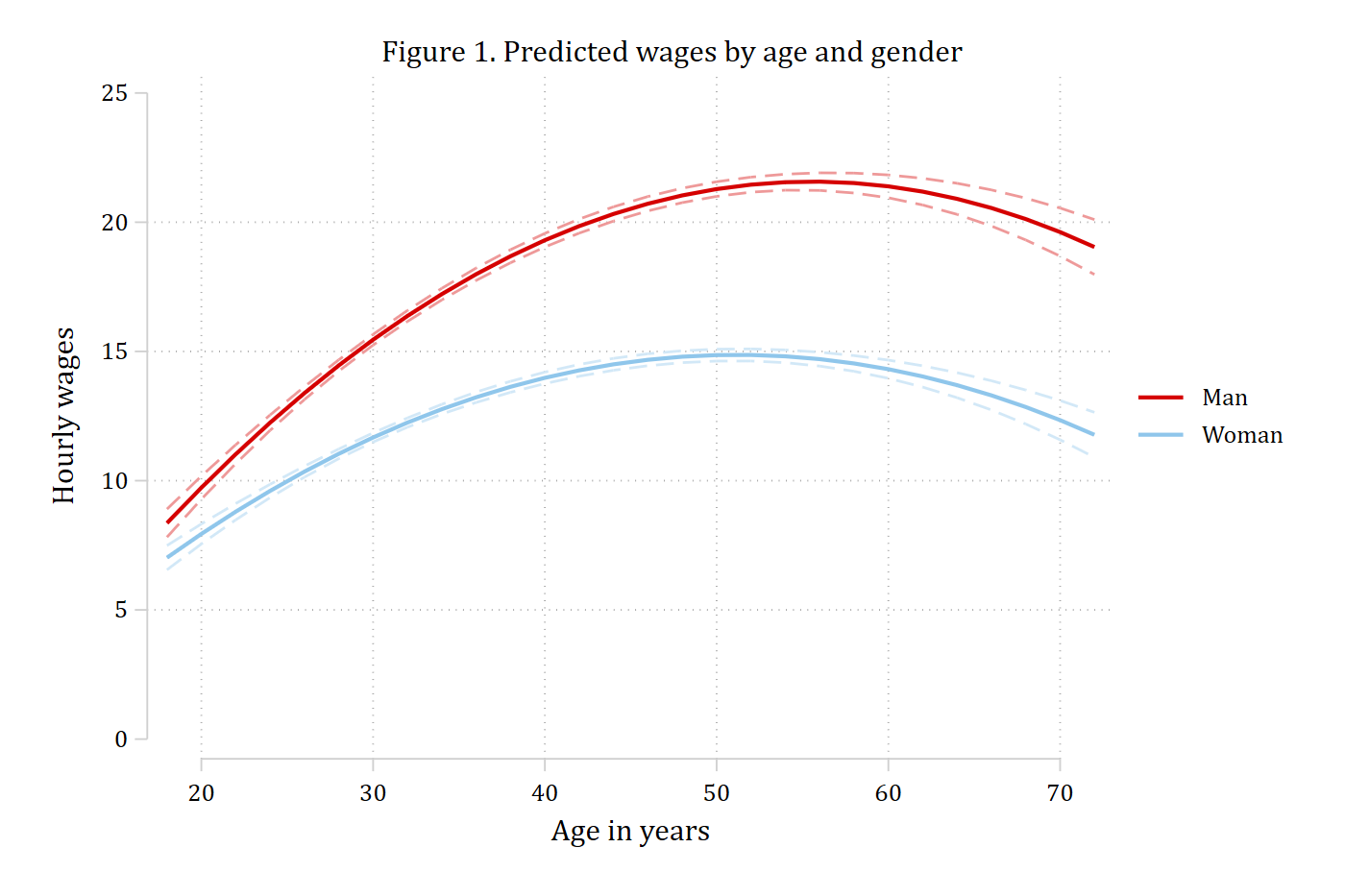
Wages rise with age and then fall, and the curves for men and women are not parallel. Whether the effect of age differs by gender therefore has to be asked at particular ages, or on average across the sample. Table 2 of the article does both.
The effect of age for men and women (Table 2)
The first row of Table 2 is the effect of aging from 25 to 30. start(age=25) puts everyone at 25, amount(5) uncentered moves them to 30, and by(woman) calculates these effects for both men and for women. The second difference – whether the effect of aging is the same for men and women – is metest 1 - 2.
mecompare age, models(regwages) start(age=25) amount(5) uncentered by(woman)Predicting: Linear prediction
Marginal effects (N_regwages=30931)
| ME # Estimate Robust SE P>|z|
---------------------------------+---------------------------------------
age + 5 (uncentered) |
Man | 1 2.628 0.089 0.000
Woman | 2 1.688 0.077 0.000metest 1 - 2 | estimate se pvalue
---------------------------------+--------------------------------
age_woman_0 - age_woman_1 | 0.940 0.109 0.000 The same test from 65 to 70:
mecompare age, models(regwages) start(age=65) amount(5) uncentered by(woman)Predicting: Linear prediction
Marginal effects (N_regwages=30931)
| ME # Estimate Robust SE P>|z|
---------------------------------+---------------------------------------
age + 5 (uncentered) |
Man | 1 -1.118 0.160 0.000
Woman | 2 -1.165 0.135 0.000metest 1 - 2 | estimate se pvalue
---------------------------------+--------------------------------
age_woman_0 - age_woman_1 | 0.046 0.206 0.823 Getting older raises wages more for men than for women in the twenties, while in the sixties the effect is negative and not statistically different across genders. An interaction that exists at one part of the range of age need not exist at another.
Absent a specific age of interest, the last row of Table 2 asks the question on average: a five-year increase from each person’s own age, averaged over the sample. Dropping start() does that.
mecompare age, models(regwages) amount(5) uncentered by(woman)Predicting: Linear prediction
Marginal effects (N_regwages=30931)
| ME # Estimate Robust SE P>|z|
---------------------------------+---------------------------------------
age + 5 (uncentered) |
Man | 1 1.158 0.039 0.000
Woman | 2 0.569 0.033 0.000metest 1 - 2 | estimate se pvalue
---------------------------------+--------------------------------
age_woman_0 - age_woman_1 | 0.589 0.050 0.000 On average, there is a difference in the effect of age for men and women.
The other side: the effect of gender across age (Figure 2)
An interaction involves two variables and has two sides. The tests above focus on the effect of age; the other side is the effect of gender. The gender gap in wages at a given age is the marginal effect of woman with age held at that value. E.g. covariates(age=(25 55)) reports it at 25 and at 55 in one table so that the two can be compared.
mecompare i.woman, models(regwages) covariates(age=(25 55))Predicting: Linear prediction
Marginal effects (N_regwages=30931)
| ME # Estimate Robust SE P>|z|
---------------------------------+---------------------------------------
woman |
Woman - Man |
age=25 | 1 -2.841 0.167 0.000
age=55 | 2 -6.805 0.209 0.000metest 2 - 1 | estimate se pvalue
---------------------------------+--------------------------------
woman_age_55 - woman_age_25 | -3.964 0.278 0.000 Women earn less than men at both ages, and the gap is significantly larger at 55. Absent particular ages of interest, a good default for a continuous moderator is its 10th, 50th, and 90th percentiles – a low, a typical, and a high value that are all in the range of the data. summarize, detail returns them and they go straight into covariates(). The joint test that the three gaps are equal is the test of interaction on this side, and the difference between the 90th and the 10th percentile is the single summary of how much the gap changes across age:
quietly summarize age, detail
mecompare i.woman, models(regwages) covariates(age=(`r(p10)' `r(p50)' `r(p90)'))
Predicting: Linear prediction
Marginal effects (N_regwages=30931)
| ME # Estimate Robust SE P>|z|
---------------------------------+---------------------------------------
woman |
Woman - Man |
age=25 | 1 -2.841 0.167 0.000
age=39 | 2 -5.192 0.168 0.000
age=59 | 3 -7.030 0.270 0.000metest 1 = 2 = 3Tests of equality
| chi2 df pvalue
---------------------------------+--------------------------------
woman~25 = woman~39 = woman~59 | 205.170 2.000 0.000 metest 3 - 1 | estimate se pvalue
---------------------------------+--------------------------------
woman_age_59 - woman_age_25 | -4.188 0.319 0.000 The full picture is the effect of gender across the whole range of age: give covariates() the range, save the results with store(), and plot them with coefplot. recast(line) connects the effects and ciopts(recast(rline)) draws the confidence interval as a band, the same look as the marginsplot figures.
mecompare i.woman, models(regwages) covariates(age=(20(5)70)) store(gap)Predicting: Linear prediction
Marginal effects (N_regwages=30931)
| ME # Estimate Robust SE P>|z|
---------------------------------+---------------------------------------
woman |
Woman - Man |
age=20 | 1 -1.789 0.275 0.000
age=25 | 2 -2.841 0.167 0.000
age=30 | 3 -3.781 0.134 0.000
age=35 | 4 -4.609 0.151 0.000
age=40 | 5 -5.326 0.171 0.000
age=45 | 6 -5.931 0.177 0.000
age=50 | 7 -6.424 0.180 0.000
age=55 | 8 -6.805 0.209 0.000
age=60 | 9 -7.075 0.291 0.000
age=65 | 10 -7.232 0.430 0.000
age=70 | 11 -7.278 0.616 0.000
. coefplot gap_regwages, vertical recast(line) ///
ciopts(recast(rline) lpattern(dash) color(*.4)) yline(0) ///
rename("^.*=(.*)$" = \1, regex) ///
ylabel(-10(2)2) xtitle("Age") ytitle("Effect of gender: women - men") ///
title("Figure 2. AME of gender across age") ///
note("Effects below zero indicate women earn less than men at that age")
graph export "fig/nli-wages-gender-gap.png", replace width(1400)file fig/nli-wages-gender-gap.png saved as PNG format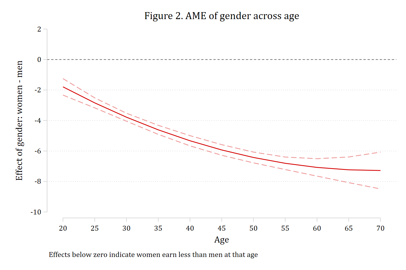
The gap is significant at every age (no interval crosses zero) and grows with age. Because these are direct tests of the group difference, the confidence intervals here say what overlapping intervals on the predictions plot cannot.