balanceplot

Plots of standardized covariate imbalance

balanceplot calculates and plots covariate imbalance for categorical or continuous treatment variables. Standardized imbalance provides a useful way to present differences across covariates even when they are measured on different metrics. balanceplot can also be used to compare covariate balance before and after matching or weighting.

The command supports factor-variable syntax and uses coefplot (Jann) to create the graphs. Continuous-treatment analyses also require the user-written polychoric command, and the examples on these pages use esttab (from estout) and psmatch2. All four are on SSC:

ssc install coefplot
ssc install polychoric
ssc install estout
ssc install psmatch2

Installation

net install balanceplot, from("https://tdmize.github.io/data") replace

The help file is also on this site.

Citation

Mize, Trenton D. 2018. “balanceplot: Stata command for plots of standardized covariate imbalance.” https://www.trentonmize.com/software/balanceplot

Background

Balance plots come from the experimental and causal inference (matching) literature. In an experiment the treatment and control groups should be “balanced” due to random assignment: the covariate distributions should be the same across conditions. When using a matching method, the pre-matched sample is imbalanced but the post-matched sample should be balanced. Despite these origins, balance plots are applicable in any analysis of groups.

Rosenbaum and Rubin (1985) proposed the commonly used measure of “standardized difference” or “bias” to quantify differences in balance across groups, which is similar to Cohen’s d:

\[ \text{Standardized imbalance} = \frac{\text{Mean}_{\text{group}} - \text{Mean}_{\text{base}}} {\sqrt{\left[\dfrac{\text{SD}^2_{\text{group}} + \text{SD}^2_{\text{base}}}{2}\right]}} \]

Values closer to zero indicate greater balance between groups.

For binary and nominal covariates, balanceplot can instead use Cohen’s h, a standardized measure of the difference between proportions:

\[ \text{Cohen's } h = 2 \sin^{-1}\!\left(\sqrt{p_{\text{group}}}\right) - 2 \sin^{-1}\!\left(\sqrt{p_{\text{base}}}\right) \]

The cohensh option uses Cohen’s h for binary and nominal covariates while continuing to use standardized differences for continuous covariates.

For a continuous treatment variable, balance is assessed using the correlation between the treatment and each covariate. balanceplot uses Pearson correlations for continuous covariates and polyserial correlations for binary indicators, including separate indicators for each category of nominal covariates. Values closer to zero indicate less association between the treatment and the covariates.

The three uses

balanceplot varlist, group(groupvar)

balanceplot varlist, contreat(varname)

balanceplot, tebalance

group() compares covariate balance across the categories of a categorical variable. contreat() plots correlations between a continuous treatment and the covariates. tebalance plots balance before and after matching or weighting, following supported teffects and stteffects commands.

Categorical covariates are specified with factor-variable syntax (i.); bare variables and c. variables are treated as continuous.

Where to start

Options runs every option of the group() form, with a graph or table for each.
Tables and stored results: table, tablefull, the formatting options, store() with esttab, and the returned matrices.
Continuous treatments: contreat().
Matching and teffects: matchweight() after psmatch2 and tebalance after teffects.
Examples from the help file runs the help file’s examples, and the help file is on the site.

A first example

The basic use of balanceplot compares standardized covariate imbalance across the groups of a categorical variable:

sysuse nlsw88, clear

(NLSW, 1988 extract)

balanceplot wage age i.married i.race tenure, group(union)

NOTE: 10 observations were excluded due to missing data on
at least one covariate, group(), or outcome() variable.


Base category = 0_Nonunion
Base selected by the 0/1 two-group default.


N used in balance calculations
- N for union = 0_Nonunion: 1408
- N for union = 1_Union: 460

graph export "fig/index-default.png", replace width(1400)

file fig/index-default.png saved as PNG format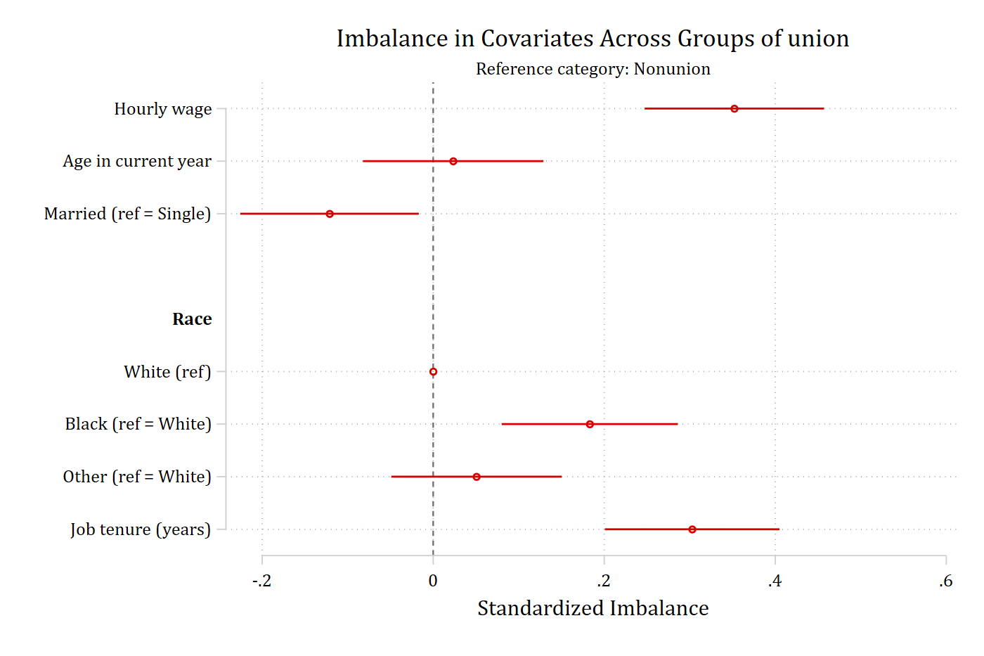

Default balance plot comparing union and nonunion workers on wage, age, marital status, race, and tenure, with 95% confidence intervals.

Each covariate’s standardized imbalance is plotted with its confidence interval, and the categories of a nominal covariate are grouped under a heading with the reference category shown at zero. The output reports the observations excluded for missing data and the size of each group.